
So this will be part one of a multi-portion series of posts. This first post will be very mathematically dense, but if you make it through, it will make the programmatic sections that much more enriched and clear.
While robots come in many different forms from autonomous cars, to drones, and even robots that swim underwater, one thing is for sure, robotic manipulators (arms) are quintessential to the study of any form of robotics. The ability for a robot to convert bytes and electrical signals to effect the world around it is one of the most amazing things about this field. With that in mind, Forward and Inverse Kinematics (FK and IK respectively for the remainder of these posts) are often some of the first things one learns when they start to learn about robotics.
Tesla’s Robotic Charger must use IK to calculate its joint configuration to properly interface with the charging port without crashing.
Before we really sink our teeth into some math, I want to present the concepts of FK and IK conceptually first, because it’s easy to lose sight of what our goals will be when the matrices and notation roll out. I am going to assume that you are reading this on some form of a screen, whether a phone/tablet or a computer monitor. I want to visually look at the top left-hand corner of that screen, and then with your free hand, reach out and touch it with your index finger. While you reach out and touch it, think about how you could have reached it from where you are right now, you probably have enough reach to touch it from the top, or the left side, maybe even perpendicular from the front side of the screen. Thanks to your reach and dexterity, you probably can touch multiple points in the environment around you from a number of ways. A lot of times, robots have the ability to reach several points in space, from multiple angles and joint configurations. This type planning to a particular point in space is what IK is all about.
Source: https://staff.aist.go.jp/eimei.oyama/hpcle.html
Planar Kinematics: Forward Kinematics
Kinematics is the study motion of [rigid] bodies without worry or concern of the forces that caused them or are involved in these motions. We will start off with a really simple example of a planar robotic arm and describe some of the forward kinematics of the arm, which will result in a relationship between a robot’s joints, and where its end effector is in space!

Three Degree of Freedom (DOF) Planar Manipulator with Three Revolute Joints, Source: Introduction to Robotics, H. Harry Asada
The image above shows a serial manipulator, which consists of links of length, that reach from joint axis to joint axis. Each joint has a name of O, A, B, and the end effector (sometimes called tool-tip/frame) is E. With these joints defined, we can now state the length of Link 1 is the distance between joint axis O and A, Link 2 has a length of the distance from A and B, and so on and so forth. If you look at the above image further, you will see that the joints can all rotate around a fixed axis and they will all cause the point, E, to move. We can now state that the position of the end effector in terms of its xₑ and yₑ components. It is also worth stating that this position is with respect to the frame of O. We can then state this relationship between the base frame and end effector frame as such:


We can validate the above equation through derivation and matrix multiplication. If you are new to matrix math and matrix representation of equations, particularly with respect to frame transformations, I highly suggest you check out this chapter from Springer’s Robotics textbook for a detailed description. For a quick recap though, we can state that the rotation, R, around the Z axis as such:

We can, therefore, state that rotation in matrix notation as:

Therefore, by example, we can describe the above planar manipulator as a set of matrix transformations for θ₁, θ₂, and, θ₃ as follows:
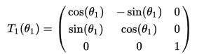
Initial Rotation around the Z- Axis of Frame O
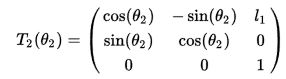
Pose of the Second Link, With Respect to the First Link, about Frame A, taking into account rotation and translation thanks to l₁.

Pose of the Third Link around Frame B. Note the inclusion of the length of the link, l₂.

Rotation of End Effector Frame E with respect to the third link. Note that since Frame E can never be anything other than inline with frame B, the value for θ will be zero and simplify to above.
We can now state that the transformation from the base frame to the end effector frame is the multiplication of each of the frame transformations between the base frame and end effector frame, that is:


Note: The letters c and s are cos() and sin().
The last step to arrive back at our initial set of equations is to recall that, the position of the end effector has an x and y component, and that our rotations take place in the z component of each frame, therefore we have:

Which gets us back to:
Planar Kinematics: Inverse Kinematics
In the previous section, we studied the relationship between joint angles and an eventual Cartesian position in space, and therefore we can create a new set of definitions and a subsequent relationship in space. We call the configuration of a robot in terms of its joint angles as “Joint Space” and we call the configuration of a robot with its end effector/tool tip in space as it’s “Cartesian Space” configuration. Below is a good graphic that shows this relationship between spaces and FK/IK.

Relationship between Forward Kinematics and Inverse Kinematics
With this relationship established, we can use the concepts and mathematics developed above to figure out the position of the end effector in space, given that we know the joint angles. The real fun begins now. How do we calculate what joint angles will give us a particular point in space if we want to move the robot to do something interesting. Recall the above planar robot, now let’s try and move to a new point in space:

The 3DOF arm is now going to try and reach a new point in space, which will require the calculation of θ₁, θ₂, and, θ₃. This will then lead to us placing the Frame E at xₑ, yₑ, ϕₑ. Source: Introduction to Robotics, H. Harry Asada
Given the above image, and assuming we know what the wrist orientation, ϕₑ, is at, we can simplify the transformation from point E with respect to O as follows. First, let’s recall the earlier results for the transformation from T1 to T4. We can simplify that by dropping off the last length, l₃, since we know what orientation we want the wrist to be in via the variable ϕₑ. We can go back and solve for the last joint angle after we have the other two joint angles. Therefore we can state that: 
and state that:
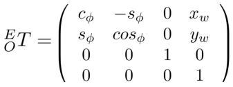
Setting those two together, gives us these equations:

We can square and add the expressions for xₑ, and yₑ and obtain:

We can continue to solve for cos(θ₂) and get:

Note, depending on which sign you decide for the sine function, will give you two different solutions. More on that later.
One down, three to go! We will now solve for θ₁:

It should be noted that if our x and y values are equal to zero, that leads to something called a singularity. The math just doesn’t work out and it doesn’t have a solution.
Now that we have these two angles, we can go back and solve for the last angle!

There it is, that would be a valid solution in joint space to reach the desired position in space. A few things to note though. First off, as we were calculating the second joint angle for Frame A (θ₂), I mentioned that depending on if we picked the positive or negative sign, it will affect the rest of our solutions, the image below shows two valid solutions due to the nature of the math, but with different signs. This type of situation is often addressed by either some level of a cost function, dependent on the initial state of the robot, to either pick the shortest path, OR if an obstacle is in the way, and the system and perceive it, to plan around it/not view it as a valid solution.
Another thing, there was a warning about joint space… if you try and run IK solutions and end up with joints in line with other joints like θ₁ could have been if it were zero, it will result in a mathematically impossible solution. Even if the robot can physically reach it, the numbers don’t play well. Just something to keep in mind.
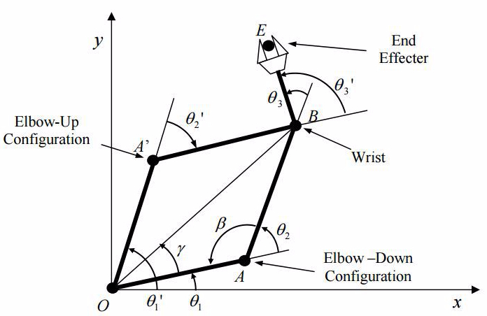
This figure shows the possibility of multiple solutions. Source: Introduction to Robotics, H. Harry Asada
In closing, this was a very simplified example in reality. Robot arms come in 6 or 7 Degrees of freedom and operate in 3D space, making it very difficult to show without some level of computational assistance and visualization… Let’s go look at something fun!
Computational Inverse Kinematics with ROS
To those who followed this post, this is the benefit of your hard work! The featured image above shows a Universal Robot (UR) planning a trajectory from one point in space to another. I am using a path planning/IK solver called MoveIt! which is a fantastic and flexible open-source package that you can use in the ROS ecosystem to plan complex robot actions. What I will be doing today is showing you how to download the standard UR packages, and use MoveIt alongside a physics simulator named Gazebo to plan some trajectories! Granted what I’m showing you here should be taken with a grain of salt. There is a lot of stuff going on under the hood, but you should at least have a better idea of some of the things that are happening thanks to FK/IK!

I begin by assuming that you will have installed ROS in its entirety as I continue with this tutorial.
First, you’ll need to clone the repo and build the repo into your Catkin Workspace by running:
$ git clone -b YOURDISTRO-devel https://github.com/atomoclast/universal_robot.git
Once that’s done, you will need to then open three terminals and launch the following three commands:
$ roslaunch ur_gazebo ur10.launch
$ roslaunch ur10_moveit_config ur10_moveit_planning_execution.launch sim:=true
$ roslaunch ur10_moveit_config moveit_rviz.launch config:=true
With everything running properly, you should see two screens open as shown in the gif above, one Gazebo simulation window, the other for Rviz. Gazebo, for all intents and purposes, is a real robot to ROS and MoveIt!, which is fantastic, because we will be trying to run it like a real robot. Simulation is an important part in modern robotics because it allows us to abstract, develop, and test higher level control without having to worry about the normal hardware gremlins that always crop up, like having emergency stops needing to be watched, and issues with the lower level controls.
In the RVIZ Window, you will need to select a Planning Library, I suggest RRTConfig, that planner works well with these arms. In future posts, I will get into planning methods and types. It may be worth checking out different planners and trying them out.
Once your planner is picked, select the Planning tab, there you will be able to grab the little orb on the tip of the robot arm, which is called an Interactive Marker. From there, you can grab it and move it freely and see the virtual robot follow, you can grab the arrows and move it in component directions and you can even grab the curved sides and change the orientation of the marker.
When you have the arm in a place you want to try and plan to, you can hit the “Plan” button, see a preview of the trajectory, then hit “Execute” and watch the Gazebo Sim as it moves!
After you’re done with that, you can play around with different configurations between planners as well as starting and ending points for the end effector. The curious reader can even follow some of the MoveIt Tutorials, and learn some more!
In my next post, I will begin to explain Jacobians, and look at MoveIt Python API to allow us to have some real control over our UR Robot! Until then, Happy Tinkering!
Liked what you saw? Subscribe for more cool how-tos, side projects, and robot stuff!
Have a comment, issue, or question? Leave a comment or message me on GitHub.

Impressive and quite thorough.
LikeLike
Loved the ROS part keep them coming!
LikeLiked by 1 person
Looks fantastic and quite thorough.
LikeLike
Amazing job. Love it. Keep it up!
LikeLiked by 1 person
Superb use of ROS for tutorial 🙂
LikeLiked by 1 person
In the introductory part you used _3x3_ homogeneous transformation matrices to describe the geometrical model of the serial manipulator. In the second part you started using _4x4_ homogeneous transformation matrices. Why don’t stick to the same notation throughout the whole tutorial?
Anyway, great tutorial.
LikeLike
Hey SebNag, thank you for reading through. Good question, the last column is because it’s rotation and translation. You’ll notice that we take into account the rotation matrix as well as translation, hence the 4×4 change. I do agree with you, i could have been more explicit about the change, or just been consistent all the way through. Thanks for reading!
LikeLike