
In my last post, we built on kinematics by introducing Jacobians for robotic manipulators. This week, I’m looking to shift a bit and start to explore mobile robots and path planning. Mobile robots are all around us now. From useful Roombas to the rise of autonomous cars, mobile robots are becoming more and more popular in our everyday lives. These robots, unsurprisingly, move around and must use an array of sensors to perceive their environments, even accounting for how these environments may change. Robots must be able to achieve specific goals, and that requires them to navigate to specific areas of interest. So, how do we go about giving robots this ability? Aside from more advanced problems like SLAM (Simultaneous Localization and Mapping), which requires a robot to construct a map while trying to estimate (guesstimate) their position in space, there are a number of well-known algorithms to plan the shortest path from a start location to a goal location in an (assumed) static map. So let’s get into it!

Amazon’s (previously Kiva Systems’) mobile warehouse robots must be able to plan a path from their current location to a goal location in order to move goods efficiently from storage to shipping. Note that a more collaborative level is also at work to ensure robots aren’t colliding, but that is out of the scope of this post.
What’s a Graph?
To answer the question of what a graph is, we turn to a branch of mathematics called Graph Theory which states that a graph is a structure that relates a set of vertices (or nodes) through edges. We can, therefore, state that a graph is an ordered pair G = (V, E), with V being the set of vertices and E their associated edges.
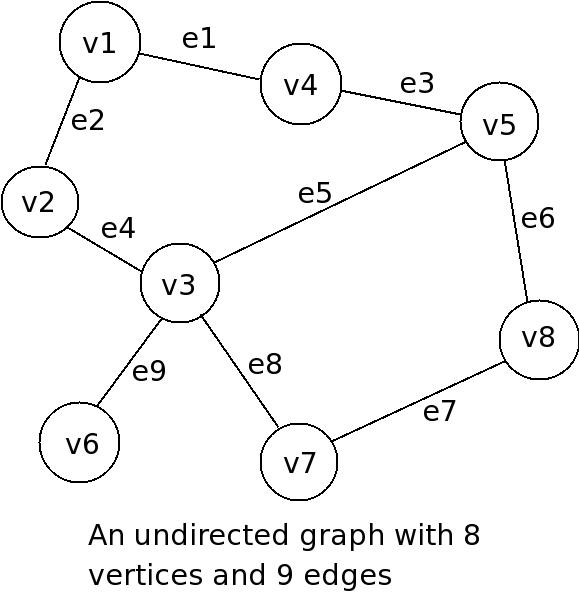
This is a simple example of a graph and shows the relationship between vertices/nodes via edges. Source: bcu.copsewood.net/dsalg/graph/diag1.jpg
This definition is purposefully general as graphs can be used to model various data structures, for instance, an Octree. Octrees have applications in things such as 3D computer graphics, spatial indexing, nearest neighbor searches, finite element analysis, and state estimation.

An Octree is a tree-based data structure with a root node that branches out into 8 children nodes that can then branch out even further. Source: https://en.wikipedia.org/wiki/Octree
In robotics especially, octrees have been leveraged via the creation of the OctoMap Library, which implements a 3D occupancy grid mapping approach. This provides data structures and mapping algorithms that not only assist in mobile robot navigation and mapping, but also helps in path planning for manipulators in cluttered environments.
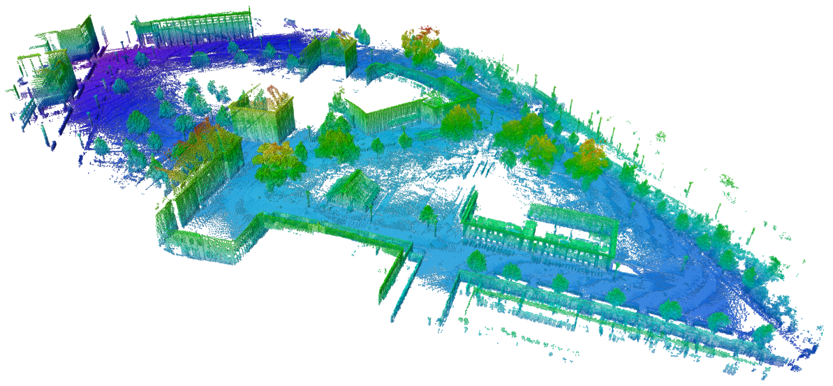
An example octomap of an outdoor environment. A map this large can be visualized efficiently thanks to the tree based structure of an Octomap. Source: octomap.github.io/freiburg_outdoor_big.png
Dijkstra’s Algorithm
Dijkstra’s Algorithm is a fairly generic way to find the shortest path between two vertices that are connected by edges. Let me present to you an interesting problem. Say that we are planning a trip with connecting flights, and we want to get from one city to another in the most efficient way, we can generate a graph like this:

An example graph relating cities and their distances from each other. Source: http://www.mcs.csueastbay.edu/~grewe/CS3240/Mat/Graph/CitySearch.JPG
Say that we wanted to plan a trip from Austin to Washington. There are several paths that we can take:
- Path A, 1560 miles: Austin -> Houston -> Atlanta -> Washington
- Path B, 2980 miles: Austin -> Dallas -> Denver -> Atlanta -> Washington
Notwithstanding the philosophical quandary regarding the merits of the journey versus the destination, if our final goal was Washington, Path A would definitely be the most desirable. The above example was solved with relative ease by looking through the graph and quickly summing up the distances between edges of our starting node in Austin and our destination node, Washington. One can also solve it by trying to count the number of nodes between the start point and end point.
Another example of a graph is a grid-based structure as shown below. This grid denotes a starting point and a goal point with several different paths that would solve the problem. In this type of graph, each square is a node (vertex) that is connected to its four surrounding neighbors via edges that have a value of one.

An example grid that shows multiple solutions to a path planning problem. Source: C.J. Taylor, University of Pennsylvania
Again, we can solve the above path planning problem by counting how many steps it would take to reach the start position from the goal, or vice versa. While this is a real planning solution (called the Grassfire Algorithm), it’s often tedious and very computationally intensive because each node must be visited to find the shortest path. This can pose a serious problem if our map is comprised of hundreds of nodes.
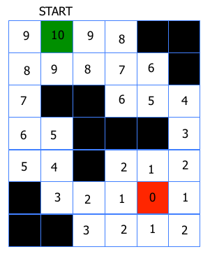
By counting the number of steps it would take to go from the goal to our starting point, we can find the shortest path. This is a very tedious process because each node must be visited. Source: C.J. Taylor, University of Pennsylvania
While the above two examples are easy to solve as humans, the real difficulty is programmatically solving these problems in a robust and efficient manner. Enter Dijkstra’s Algorithm, which was developed by Edsger W. Dijkstra. Djikstra was incredibly influential in the rise of the field of computer science, both from theoretical and implementation/engineering perspectives. Dijkstra began to try and solve the path planning problem in 1956, and then published his solution three years later detailing out his algorithm. The above example started at the goal and radiated outwards until it visited every node, counting each step along the way. Djikstra proposed a similar solution, but one that starts at the first node and grows out towards the goal. Using “Big O” notation, we can state that the time it will take to run this algorithm increases linearly with the number of edges, meaning: O(|V|), where |V| is the number of nodes/vertices on the graph.
We can describe the algorithm in pseudo-code as follows:
For each node, n, in the graph:
n.distance = InfinityCreate an empty list
start.distance = 0, add start to listWhile list not empty:
Let current = node in the list with the smallest distance, remove current from listFor each node, n that is adjacent to current:
if n.distance > current.distance + length of edge from n to currentn.distance = current.distance + length of edge from n to currentAdd n to list if it is not there already
Using the above pseudocode, we can find the shortest path from Austin to Washington in a programmatic manner. Below is a great animation I found that really shows the algorithm in action:
Dijkstra’s Algorithm on a graph. Source: https://en.wikipedia.org/wiki/File:DijkstraDemo.gif
Computational Complexity of Dijkstra’s Algorithm
Djikstra’s algorithm is an improvement to the Grassfire method because it often will reach the goal node before having to search the entire graph; however, it does come with some drawbacks. On occasion, it may search nearly the entire map before determining the shortest path. That can be both tedious and time-consuming depending on the number of nodes to be searched. We can estimate worst case performance by using “Big O” notation, O(|V|²).
One can improve the efficiency of Dijkstra’s Algorithm by using a clever data structure known as a priority queue. This particular data structure is different from a normal queue data structure because instead of the standard “first in, first out” implementation, it will pop the values based off of the associated priority.

Simple visualization of a priority queue. Source: http://pages.cs.wisc.edu/~vernon/cs367/notes/11.PRIORITY-Q.html
This simple data structure can help reduce how quickly the computational load increases. This rate can be described as O((|E|+|V|)log(|V|)). Where |E| and |V| are the number of edges and vertices (nodes) respectively.
Dijkstra’s Algorithm in Python
This week’s code snippet is purely Python and is a modified implementation of Dijkstra’s that I used for a mobile robot. To get started, let’s clone the repo locally on your machine:
$ git clone https://github.com/atomoclast/realitybytes_blogposts.git
With that cloned locally, you should be able to run it by navigating to:
../realitybytes_blogposts/pathplanning/
and running:
$ python dijkstra.py
You should see a window open up similar to the one below showing an occupancy map. The darker blue color is free space, the lighter blues are walls/obstacles. The yellow square is the starting node, and the orange square is the goal node. You will see that we will begin searching around the starting node. Once a node is searched, it will become aqua blue, and the search will keep radiating out until the goal node is found. Once that is found, the shortest path is calculated and visualized in red!
There are three maps that will run in sequence if you just run the command above. The first two will iterate and find the goal, while the last one will fail because the goal node is blocked off from the start node via a wall. This was intentional to test my implementation and how it will handle such an event.
Dijkstra’s Algorithm in action for an Occupancy Map. It will search until the goal is found and then visualize the path in red.
Once you’ve run the out of the box code, let’s really look into it and see what’s going on. The function itself takes five arguments and returns a discrete path or a failure boolean:
def dijkstras(occupancy_map, x_spacing, y_spacing, start, goal)
The variable occupancy_map is a NxM numpy array of 0s and 1s that represents the locations of walls and obstacles as well as free space in the world. The variables x_spacing and y_spacing are parameters that represent the space between adjacent columns and rows respectively. I told you that this was implemented on a real robot, so when a map was explored and built up, we discretized the metric values into nodes on a graph using the following relationships:
x = (j + 0.5)*x_spacing

y = (i + 0.5)*y_spacing
The starting and goal positions are a 3×1 numpy array of (x, y, theta) with theta being the orientation of the robot in space. We don’t need to worry too much about any constraints on theta because we assume the robot is holonomic. Holonomic means that the robot is like a Roomba. It can rotate around its z-axis, without having to move in the x or y directions. This makes planning much easier for this type of robot vs. a nonholonomic robot, like a car.
Two very useful variables that I have defined in the Python file are DEBUG and VISUAL. If DEBUG is set equal to ‘True’, then the print statements within the code will be displayed on the terminal during every iteration. If VISUAL is set to ‘True’, then the animation windows will be created and displayed as the algorithm runs. Use them as you see fit to play around with maps, adjusting the start and goal positions. You can also change the dimensions and “landscape” of the occupancy maps that you pass to the algorithm. Again, I really urge that you take the time to read through the code, the comments, and play around with Dijkstra’s Algorithm to get a good feel for it!
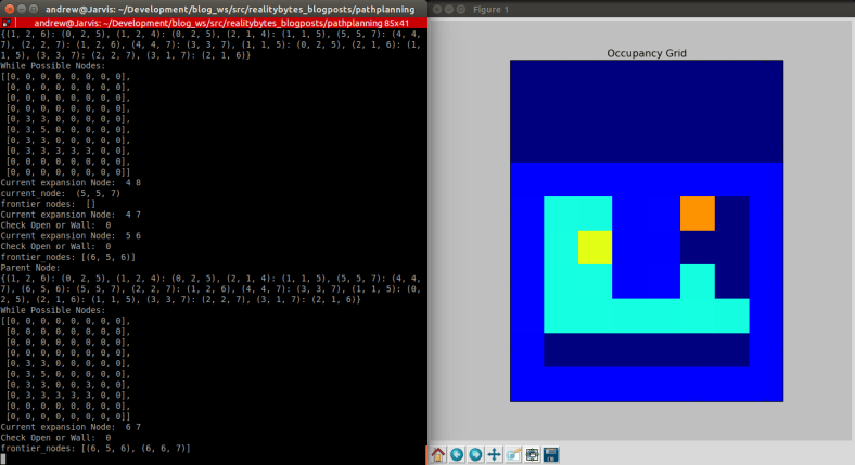
Setting the DEBUG and VISUAL flags to True will show the animation as well as the data flow behind the scenes on your screen.
In future posts, we will look to an extension of Dijkstra called A* (pronounced “A Star”), and how it uses one relatively simple trick to make Dijkstra a little more efficient.
Until next time, happy robotting!
Liked what you saw? Subscribe for more cool how-tos, side projects, and robot stuff!
Have a comment, issue, or question? Leave a comment or message me on GitHub.
Featured Image Source: http://www.astro.mech.tohoku.ac.jp/~ishigami

Simple and thorough, thank you. Well done!
LikeLiked by 1 person