Graph-Based Path Planning: A*

August 17, 2018Atomoclast Leave a comment

A while back I wrote a post about one of the most popular graph based planning algorithms, Dijkstra’s Algorithm, which would explore a graph and find the shortest path from a starting node to an ending node. I also explored the very fundamentals of graph theory, graph representations as data structures (see octrees), and finally, a python implementation that animates the search process for several example graphs. If you haven’t read that yet, I urge you to please check that out, because I will be continuing the discussion assuming some prior knowledge with the subject.

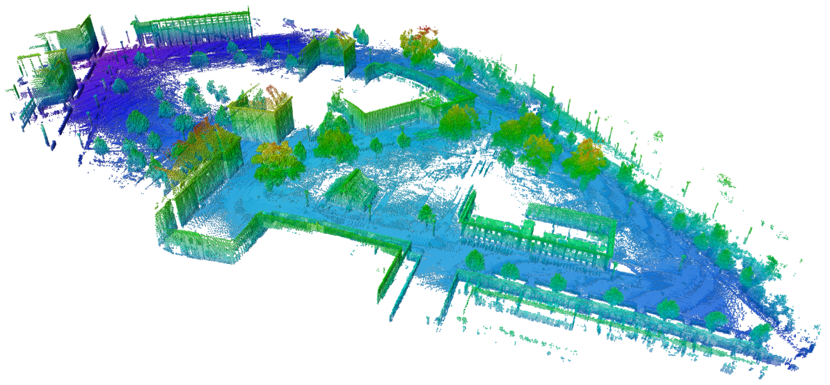
An example octomap of an outdoor environment. A map this large can be visualized efficiently thanks to the tree-based structure of an Octomap. Source: octomap.github.io/freiburg_outdoor_big.png

Dijkstra vs A*

Dijkstra is novel because it begins exploring from a starting node and continues until it reaches the ending node. It then identifies the list of nodes that connect the end node to the start as one single path. This means that Dijkstra works by exploring nodes in order based by their distance from the starting node. To put it another way, this means that it will equally explore nodes that are farther from the goal as well as nodes closest to the goal as it expands outwards from the starting node. As one can imagine, that can become computationally expensive as our graph representation of our world grows.

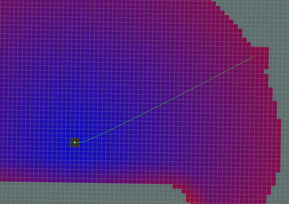
Example of Dijkstra’s Algorithm attempting to go from a start node to a goal node. See how it has to expand out almost the entire distance of the path in every direction before it finds the goal? Source: wiki.ros.org/global_planner

So, in 1968, an AI researcher by the name of Nils Nilsson tried to improve on this planning approach for Shakey the Robot, a prototype mobile robot from SRI. The algorithm that was developed for Shakey is what is now known as A* (pronounced ‘A Star’). A* tries to improve on Dijkstra’s Algorithm by focusing only on exploring nodes that bring us closer to our goal. This greatly improves our speed of finding the shortest and most direct path.

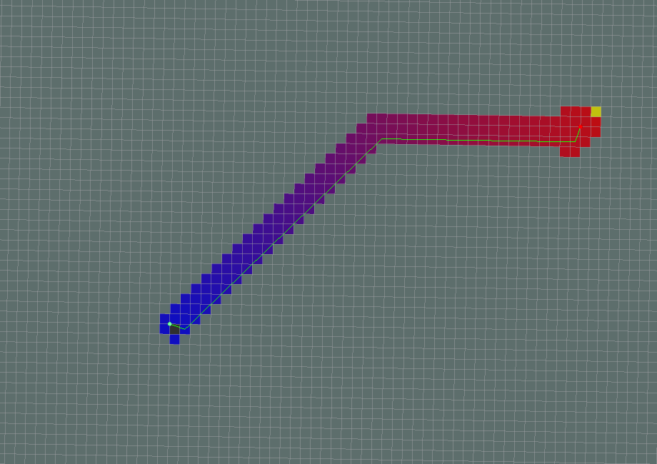
The same path planning problem as shown above, but look at how quickly the goal is found? With the use of some forcing heuristic, we ensure that we only expand nodes that drive us towards the goal node. Source: wiki.ros.org/global_planner

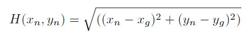
The way A* does this is via the introduction of a heuristic function that guides the node expansion towards the goal. Our heuristic functions will be used to create a correlation from every node in the graph to a non-negative cost value. Heuristic functions (represented as the function H below) must satisfy two basic criteria:

H(goal) = 0
For any two adjacent nodes x and y:
1. H(x) <= H(y) +d(x, y)
2. d(x, y) = weight/length of edge from x to y

The notion that our cost is zero at the goal node helps address the issue described above that when we explore from the starting node, we have no real direction. So if we have some extra value that can assess if an explored node will bring us closer to the goal, we improve our search time. Following these two criteria, we can ensure that every node will be less than or equal to the length of the shortest path from node n to the goal. Two of the most popular examples of heuristics are the Euclidean Distance, and Manhattan Distance from any node, n, in the graph to the goal, g, in the graph. We can, therefore, say, given any node, n, at (xₙ, yₙ) and a goal, g, at (x_g, y_g):

Euclidian Distance
Manhattan Distance

With this heuristic now in place, we can update our previous Dijkstra algorithm as follows:

For each node, n, in the graph:
- n.distance = Infinity, n.g = Infinity
Create an empty list
- start.distance = 0
- start.f=H(start)
- add start to list
While list not empty:
- Let current = node in the list with the smallest f value, remove current from list
- If (current == goal) return Success
- For each node, n that is adjacent to current:
  - if n.g > (current.g + cost of edge from n to current
    - n.g= current.g+ cost of edge from n to current
    - n.f = n.g + H(n)
    - n.parent = current
    - Add n to list if it is not there already

A* Python Example

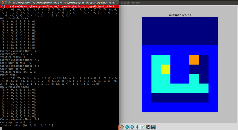
In keeping with my previous post on Dijkstra’s Algorithm, I have written a quick Python example to illustrate the above algorithm.

To get started, let’s clone the repo locally on your machine:

$ git clone https://github.com/atomoclast/realitybytes_blogposts.git

With that cloned locally, you should be able to run it by navigating to:

../realitybytes_blogposts/pathplanning/

and running:

$ python a_star.py

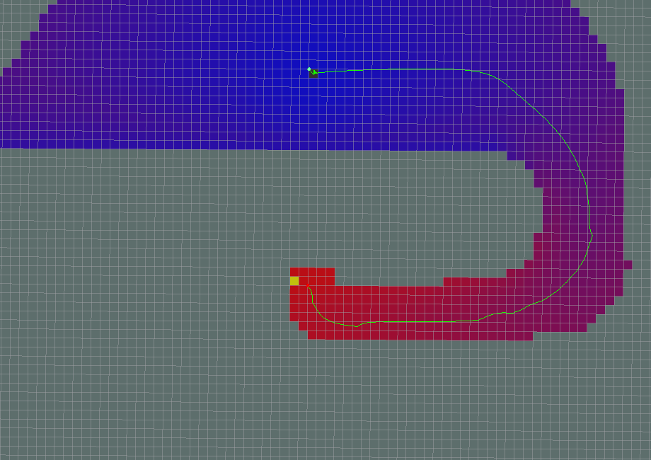
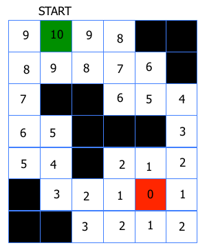
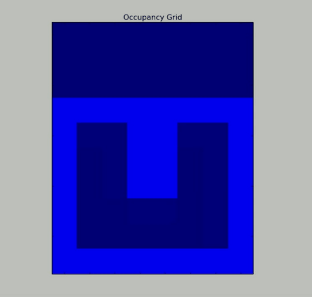
You should see a window open up similar to the one below showing an occupancy map. The darker blue color is free space, the lighter blues are walls/obstacles. The yellow square is the starting node, and the orange square is the goal node. You will see that we will begin searching around the starting node. Once a node is searched, it will become aqua blue, and the search will keep radiating out until the goal node is found. Once that is found, the shortest path is calculated and visualized in red.

A* Algorithm in action for an Occupancy Map. It will search until the goal is found, then visualize the path in red.

In the above example, there is a large L shaped wall that would prevent the quick expansion of a Dijkstra approach. That method would have to wrap around the wall and search nearly the entire map before it found the goal. Alternatively, our A* searches grow towards the goal until it is reached, with very little concern for nodes that take us away from the ending node.

In the example map code, you can see that we define a test_grid variable as a list of lists where ‘0’ indicates an open node and ‘1’ indicates an obstacle:

    test_grid = [[0, 0, 0, 0, 0, 0],
                 [0, 1, 1, 1, 1, 0],
                 [0, 1, 0, 0, 0, 0],
                 [0, 1, 0, 0, 0, 0],
                 [0, 1, 0, 0, 0, 0],
                 [0, 1, 0, 0, 0, 0],
                 [0, 1, 0, 0, 0, 0],
                 [0, 1, 0, 0, 1, 0]]

We then define the start and end nodes as a list of [x, y] node positions (starting from 0). Using this basic format, you can challenge yourself to create different maps to test your A* Algorithms.

Another interesting thing is our heuristic function, which will calculate how far each node is on the graph from our goal node. For a map this size, calculating the cost from the goal to each surrounding node costs very little, but for larger robotic applications, it makes more sense to calculate the heuristic at every iteration of the loop for computational efficiency.

What makes this A* implementation especially intriguing is the way we handle the heuristic value in our loop. As shown below:

    
for i in range(len(delta)):
    x2 = x + delta[i][0]
    y2 = y + delta[i][1]
      if len(self.grid) > x2 >= 0 <= y2 < len(self.grid[0]):
          if closed[x2][y2] == 0 and self.grid[x2][y2] == 0:
              g2 = g + cost
              f = g2 + self.heuristic[x2][y2]
              open.append([f, g2, x2, y2])
              closed[x2][y2] = 1
              delta_tracker[x2][y2] = i

In this loop, we will search through every possible orthogonal direction, and then calculate the f value as described in the pseudo-code above, which is just the running cost + the heuristic cost. Once our cost is found for the explored node, we add it to a running list of possible “open” nodes from which we pick the lowest f value on the next iteration, thus bringing us closer to the goal.

That’s it. That’s what makes A* such an amazing yet powerful algorithm!

Where to go from here:

If you are still curious about playing with some code, I challenge you to upgrade my Dijkstra’s code to A*, since I decided to go a different route with my example.

If you want to look at other examples of A* in Python, check out Python Robotics’ A* Example.

A* ROS Example

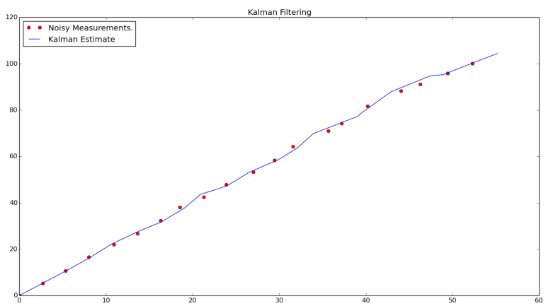
The ROS Navigation Stack is a set of software packages that make path planning and motion control (more on this in a coming post) as simple as possible for differential drive and holonomic wheeled mobile robots. There are multiple packages in this stack to help with everything from building up Cost Maps with costmap_2d to localization with packages such as amcl, which is an adaptive Monte Carlo Localization approach. Monte Carlo Localization is the process of using a known map and sensor measurements to localize where a robot is with a high degree of confidence using something called particle filters (see my other post about Kalman Filters for some motivation on the state estimation problem, PFs are just another type of filter). The most pertinent portion of the stack for Grid-Based path planning will be the global_planner package.

Source: wiki.ros.org/navigation?action=AttachFIle&do=get&target=nave_comic.png

global_planner

This package uses an implementation of A* for a fast, interpolated global planner for navigation via a discretized map. There are other implementations like a traditional Dijkstra planner that are available for configuration during launch, but the A* is undoubtedly faster.

Example A* path. Source: http://wiki.ros.org/global_planner?distro=melodic

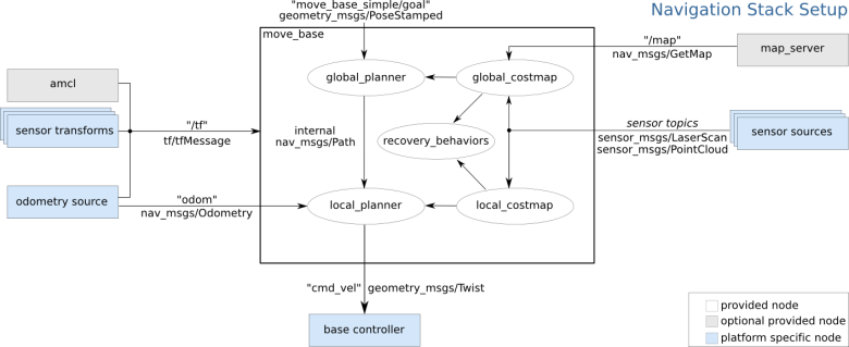
While this provides a high-level plan through a map, the question remains of how the robot’s base frame must be controlled taking into account local obstacles such as corners of walls and stand-alone objects. The move_base package provides such a feature. Once the global planner searches and publishes a plan, this package will then take that plan and link the global/local planners with an actual controller. Below is a graphic showing how the move_base node subscribes and publishes to various topics for a differential wheel robot.

Enter a caption

Looking at the source code directly on the ROS Navigation Github, you can see the source code for the global planning package has multiple source files, one of which is devoted solely for A*. The source script shows the implementation of the AStarExpansion class. The real planner is in AStarExpansion::calculatePotentials(), which will take in a starting pose, an end pose, and then iterate through a potential field and add each node it expands to a queue until the expanded node reaches the goal. If it does not find a goal, it returns back a ‘false’.

    
bool AStarExpansion::calculatePotentials(unsigned char* costs, double start_x, double start_y, double end_x, double end_y,
                                        int cycles, float* potential) {
    queue_.clear();
    int start_i = toIndex(start_x, start_y);
    queue_.push_back(Index(start_i, 0));

    std::fill(potential, potential + ns_, POT_HIGH);
    potential[start_i] = 0;

    int goal_i = toIndex(end_x, end_y);
    int cycle = 0;

    while (queue_.size() > 0 && cycle < cycles) {
        Index top = queue_[0];
        std::pop_heap(queue_.begin(), queue_.end(), greater1());
        queue_.pop_back();

        int i = top.i;
        if (i == goal_i)
            return true;

        add(costs, potential, potential[i], i + 1, end_x, end_y);
        add(costs, potential, potential[i], i - 1, end_x, end_y);
        add(costs, potential, potential[i], i + nx_, end_x, end_y);
        add(costs, potential, potential[i], i - nx_, end_x, end_y);

        cycle++;
    }

    return false;
}

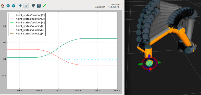
Example with ROS/Gazebo:

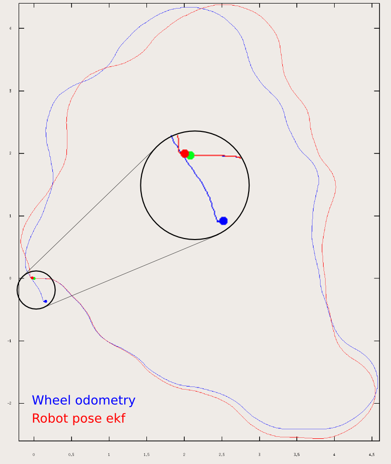
Using our trusty Turtlebot simulator and a previously explored map, we can have Turtlebot plan a global path, then navigate to that goal on the map with a Monte Carlo Localization node to provide a Particle Filter/Estimate of where the robot exists in the map and a controller to actually move the base frame of the robot.

To install the package, we will run:

    
$ sudo apt-get install ros-[YOURDISTRO]-turtlebot-stage

Then once that is installed, run:

    
$ rospack profile # Update our ROS package lists to find our new package.
$ roslaunch turtlebot_stage turtlebot_in_stage.launch

If everything loads successfully, you should be prompted with an RViz window similar to this:

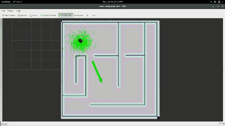
RViz window showing Turtlebot Navigating towards a goal.

In the gif above, you see the robot was given a pose, an (x,y) position in space and an orientation via the red arrow that the local planner and controller are now using. The faint red line is the output of the A* planner and the square grid around it is how the local planner is following the desired trajectory from the global planner.

To give our robot a goal, we will click the button labeled “2D Nav Goal”, and click anywhere on the map, and drag in the direction we want it to have its final orientation. From there, you should see the robot move towards the goal as shown below:

A* is an incredibly powerful algorithm that not only has applications in path planning for mobile robotics but also for general Artificial Intelligence, including the problem of semantic parsing using stochastic grammars in Natural Language Processing! It really makes you appreciate how simple ideas can find usage in world-changing applications.

Until next time, happy robotting!

Liked what you saw? Subscribe for more cool how-tos, side projects, and robot stuff!

Have a comment, issue, or question? Leave a comment or message me on GitHub.

References

Computer Vision/Perception: Structure From Motion

May 10, 2018May 10, 2018Atomoclast Leave a comment

Hey strangers! I know it has been a while since you last heard from me. A lot has been going on the last six months or so…I moved halfway across the country to start a new robotics job and I also got accepted and began an MS program online with Georgia Tech! Needless to say, I’ve been a bit swamped with all of that. I’m back now with an interesting post that started as a school project and has now developed into a side project due to my interest in the subjects related to the Structure from Motion problem.

In several of my previous posts, on path planning and state estimation, I began to mention the SLAM (Simultaneous Localization and Mapping) problem in robotics, which is often considered one of the cornerstones in truly autonomous robotics. SLAM is a very complex problem, and this post is barely going to scrape the surface of it, but I will begin to talk about the mapping portion of SLAM by talking about the Structure from Motion algorithm that has been used in many different applications outside of just robotics, such as GPS applications such as Google Maps, and surveying with drones for visual inspection. Let’s begin!

This is an example Pointcloud that was generated using the four images on the right.

Pinhole Camera Model

To begin this discussion, I’m going to quickly go over the pinhole camera model. This is just to explain some important jargon that is required for us to talk about converting things from physical space into images. Camera’s were conceptually conceived via the concept of the camera obscura, which means “dark room” in Latin, really showcases how light from a scene can enter a singular point of entry, the pinhole, and produce a virtual image on the other side of the wall.

An example illustration of a Camera Obscura. Source: https://www.photoion.co.uk/blog/camera-obscura/

I only bring this up, because the modern camera model we use in computer vision is not far from this simple physical phenomena. The image below details the process of how a real point/feature in space get transformed into a pixel in an image:

../../../_images/pinhole_camera_model.png

The blue arrow, P, represents some point in Cartesian Space that produces some pixel, (u,v) in our image. This point in real space gets translated into the pixel in our image via the intrinsics of the camera: the focal length of the lens, field of view and the distortion of the physical lense (nothing is ever manufactured perfectly) Source: https://docs.opencv.org/2.4/_images/pinehole_camera_model.png

We can describe this process mathematically as follows:

This equation is the basic format of the pinhole camera model. It relates 3D points to 2D pixel space. Note that R and t are a 3×3 rotation matrix and a 3×1 translation matrix respectively.

The first matrix on the right-hand side of the equation is referred to as the camera’s intrinsic parameter matrix. This has the focal length in vertically and diagonally via the f parameters and the optical center of the image cx and cy. This matrix describes the camera’s physical properties in “pixel” coordinates. The cx and cy values are the pixel values in the image that sit along the optical axis above. More often than not, it is pretty close to half the pixel width and height respectively, but due to manufacturing tolerances, it may not be exactly in the center of the image due to radial distortions as shown below. The focal length expressed in pixels is derived from the field of view and the lens’ physical focal length. One can obtain a camera’s intrinsic calibration matrix using a calibration process with a known checkerboard pattern as detailed in this tutorial.

Example of radial distortions from imperfect lenses. Source: https://docs.opencv.org/2.4/_images/distortion_examples.png

The [R|t] portion of the above equation is often called the joint rotation-translation matrix, which is also referred to as the “extrinsic” parameters of the model. We can think of the intrinsic calibration as the “internal parameters” to the camera and the “extrinsic parameters” as the “external” configuration of the camera. So this relates our camera back to a pose in space. You can find more information about rotation matrices and translation matrices in my kinematics tutorial if you want a refresher. Fundamentally, the rotation-translation matrix correlates a point (x, y, z) to a coordinate with respect to the camera. You can find a great write up on the OpenCV website via this link for more information.

Pivoting a bit, we can now talk about how we can build pointclouds with stereo camera rigs from a theoretical sense to help instill a sense of how we can use these physical camera parameters to build 3D clouds. If we had two calibrated cameras that were pointing the same direction, with some distance between the cameras in a purely horizontal sense, we can actually find interesting features in each pair of images and calculate where that point is in space with some simple geometry.

The ZED Stereo Camera is an off the shelf system from StereoLabs. Source: http://www.stereolabs.com

Now if we found an interesting feature in the left image and right image, we can use triangular relationships to find how far that feature is from the camera as shown below. While this is a simplification of the process, it shows how the parallax phenomena helps us calculate differences between the images to build our triangle. Parallax is when you find a feature in two images, but their horizontal locations are different, meaning that they’re along the same vertical line, but not the same horizontal line. You can observe this quickly by holding your hand out in front of your face, and close one eye while leaving the other eye open then swapping. You will see your hand seems to “shift” from the left or right as your switch eyes. For more detail on the mathematics and mechanics of stereo, follow this link.

A simple example of stereo camera triangulation. Source: https://www.cs.auckland.ac.nz/courses/compsci773s1t/lectures/773-GG/topCS773.htm

Recovering Camera Poses

In the above section, we began to detail how a camera’s pose (position and orientation) in space as well as it’s internal parameters produces discrete images for us. We then went over how we can find a point in 3D space with two cameras taking two different images. Structure from Motion operates in the same manner at a high level, but instead of having two images taken at the same time, with some distance between them, we will try and reconstruct these points by finding these matching keypoints between two images that were taken from different positions at different times. We essentially try to build a time-varying stereo camera rig!

So how do we do this? Well, we can do this two ways: by comparing each image with every other image in an image stack, or by using a video stream (think from a small robot or drone) and tracking keypoints as they move between sampled frames using optical flow. For my current example, we used an unsorted approach, where each image was compared against the others, and that’s how I will continue to describe it. I do think that optical flow is how I will probably improve my approach so I can use it with my drone in the future, but I digress.

Comparing each image in an image stack with another is the approach that was originally used in the Photo Tourism research paper published in 2006 that resulted in a software package known as Bundlr. This approach attempts to find matches between images, and then recover a camera’s pose in space by estimating the Essential Matrix via matched features, as shown below. This matrix is a 3×3 matrix that relates the points in the two images and from there, we can calculate the Fundamental matrix, which is what we really care about because it returns to us a rotation matrix, R, and a translation matrix, t.

Matches found between two images of the building scene from the example above.

We can recover these points in space because we already know some stuff about the camera: the focal length and the principal point (cx and cy). Since the focal length and optical center of the image are based on real physical measurements, and with the pinhole camera model above, we know how physical points are captured as images, we can do some math to try and solve for what these points are in space.

Where:

x and x’ is the (u, v) pixel location of the keypoint in the first image and second image respectively.
K is the calibration matrix consisting of the focal length and principal point coordinates of our camera.
E is the Essential Matrix

We use a Singular-Value Decomposition (SVD) method to solve the above equation. An interesting note to be made: there are a few methods to calculate the essential matrix, a 5-point method, and an 8-point method that uses 5 and 8 point pairs respectively. Algorithms such as RANSAC (Random Sample Consensus Algorithm) can provide many more pairs and help us have a more robust solution by having more points to triangulate on.

Graphic visualizing the Essential Matrix between two images. Source: imagine.enpc.fr/~moulopn/openMVG/Essential_geometry.png

In the implementation shown in the example above, a 5-point method is utilized to estimate the essential matrix, and that comes with the caveat of ambiguity in the scale of our images. At the end of the day, we won’t know the scale of the differences between images with respect to physical translations so our pose estimate will be relatively correct because or orientations are correct, but we can get around this by making the assumption that the “scale” factor is what is calculated between the first image pair. Note that this is a major drawback to using SfM for map building for motion planning and so on in robotics. There will need to be some external sensor that is utilized for some form of sensor fusion to recover this scale such as an IMU.

Bundle Adjustments and Triangulation

When we used the essential and fundamental matrices to estimate our pose in space, we did it with keypoints, while this is sufficient when we take two images, we haven’t leveraged the constraints that arise when we compare every image with each other and the features that are matched across every image in the image set, for example, the building above has a large overlap in matching keypoints that can improve our statistical confidence in our derived poses in space. This is where the bundle adjustment comes into play! What a bundle adjustment does is treats the entire problem space as a giant nonlinear least-squares problem! Where we try and take the camera poses, the 3D points we can match between the images, and intrinsic matrix, K, and compare them with every other image in the image stack and arrive at one singular solution that is true across all images. Again, to keep this post high level and conversational, I won’t get into the underlying mathematics, but one of the most popular methods is the Levenberg-Marquardt Method. Now thankfully for us, there are a number of libraries that have this implemented for us so this really simplifies the problem for many developers and users like us! Two bundle adjustment library options are SBBA and GTSAM.

Point Triangulation across multiple images. Once we find our poses in space, optimize our estimates of those poses via a bundle adjustment, we can then triangulate matches in space to build up a high density pointcloud for us to reconstruct a scene from images! Source: imagine.enpc.fr/~moulonp/openMVG/Triangulation_n_geometry.png

Once we’ve optimized our poses in space, we can now triangulate these points in a (hopefully) dense pointcloud artifact! To triangulate these points, we use these known camera poses, our scale factor, and matches to produce our 3D points. A popular way to produce these files is to use a program called PMVS, which is used by Bundlr and several other pointcloud generation pieces of software.

A Structure from Motion Pipeline in C++

As shown above, I have begun to tinker around with a SfM pipeline and have used it on a few image sets with some varying results. You find the source code over on my github.

The software pipeline is as follows:

Estimate Camera Intrinsics
1. An initial camera intrinsic matrix is required as arguments for the main cSfm executable. While one can calibrate a camera or use images from a calibrated camera with known intrinsic, I wanted to keep it flexible enough for any type of images to be passed into the main pipeline of the code. For most of my own images from my own camera, I assumed the center of the image was the width and heights divided by two. I then wrote a simple Python script that takes in the width of the image, the focal length in mm, and the Field Of View to estimate the focal length in pixel space. The code can be found in calculate_focal_length.py
Find Keypoints in each Image
1. From this point on, this is all automatically computed in the compiled C++ executable. Iterate through N images, and find keypoint matches in the rest of the N-1 images. Store these keypoints in a Structure for Motion Object used to ensure that every keypoint that is found is tracked throughout the pipeline of the images. As can be seen, there are a number of good matches, but some false-positives as well.
Triangulate Points Between Images
1. Using OpenCV, we then used these maps of vectors to triangulate the camera poses from matches between images, then we can use those poses to recover structure. Via triangulation. First, we find the Essential Matrix, which helps us calculate the point correspondence between two poses at the same point in space by finding the translation and rotation [R | t] from the second camera with respect to the first. The OpenCV function cv::findEssentialMat is utilized. We then take that matrix to find our poses in space using cv::recoverPose.Since this is a monocular approach, our rotation will be correct, but the scale will probably be off, so we find our scale by calculating vector length between matching keypoints. This is done while we use the cv::triangulatePoints function.
Bundle Adjustment (BA)
1. BA is the parallel process of refining triangulated points in space as well as the camera poses in space. It is a refinement process that helps us make coherent sense of the camera poses in space with some statistical confidence due to the inherent stochastic nature of our sampling. The way we go about this is to use the camera points we triangulated and the poses we recovered. While there are a number of algorithms that can be used, the Levenberg-Marquardt algorithm is one of the most popular, and GTSAM provides a very fantastic implementation of it via: gtsam::LevenbergMarquardtOptimizer
Prepare Post BA Camera Estimates for PMVS2
1. Once the bundle adjustment has been run on all of our triangulated points and poses, we will prepare those estimates in a format for PMVS to use. This requires several system calls to produce directories and populate them with images in the format that PMVS expects, and the corresponding Projection Matrix. This P matrix is what relates the camera with respect to an origin coordinate in space.
Utilize PMVS to create the Pointcloud
1. Patch-Based Multi-View Stereo is its own compiled piece of software, but it is automatically called via system calls in the cSfM executable. It looks in the local directory for the output/ directory that was generated in the last step, and takes those Projection matrices and the corresponding images, and stitches them together into the final pointcloud .ply file.

Building the Software

To build it, you will need to have GTSAM setup on your local machine. I used version 4.0.0-alpha2.

To clone it locally on a Linux machine by running,

git clone https://github.com/atomoclast/cSfM.git

From there navigate to the root of the directory:

cd path/to/cSfM

and build the executable by running:
mkdir build cd build cmake .. make

You should then see a cSfm executable now in the build directory.

Usage

To use cSfM, you will need to have a directory containing several images of your item of interest. You will also need to pass in the FULL path to a text file that contains the name of the images in the same folder you wish to build the pointcloud of, the focal length of your image (in pixels), the center of your image in x and y.

If you are using a calibrated camera, this should be easy to find as elements in the resultant distortion matrix.

However, if you are using images from a smart phone/uncalibrated camera, you can estimate these parameters.

To calculate the focal length of your image, I have written a simple helper Python script. The way you use that is as follows:

python calculate_focal_length.py [pxW] [f_mm] [fov]

where:

pxW is the width of the images in pixels.
f_mm is the focal length of the camera that was used to capture the image in [mm].
fov is the camera’s Field of View in degrees.

To get this information, one can look at the EXIF metadata that their images should have.

This should print out a relatively accurate estimate of the focal length of your images in pixel space.

For a rough estimate of the center of the image in x and y, you can use this rough estimate:

cx = PixelWidth/2
cy = PixelHeight/2

This should be accurate enough, as the algorithm will attempt to calculate a more accurate camera matrix as it triangulates points in space via the bundle adjustment.

Assumptions and Caveats

This is still a first attempt at SfM. SfM is a very complex problem that still has a lot of research conducted on how to use different cameras and different improve results. That being said, here are some thoughts and tips to get good results:

Scale down your images. This pipeline does not use a GPU based method to calculate poses in space via triangulation, so it may take a long time.
Try and use images that have large overlaps in them. Right now the pipeline matches keypoints across all the images, so if there is not enough overlap, it will struggle to recover camera poses.
Use a few images at first to test things out. Do not overestimate how computationally expensive it becomes as the size of images and volume of the image stack increases.

Examples and Results

This was one of the first simple image sets I used to test and debug my code. It is a corner of my desk at work. I figured the contrasts in colors helped with debugging false positives for
Link to video with rotating pointcloud.

This was an small group of photos taken of our Harry Potter Book Collection with some Harry Potter Bookends.
Link to video with rotating pointcloud.

A series of pictures were taken by a local pizzeria. I ran the program with the full image set, and then with only 3 images out of curiosity. The full image set created a much fuller “face” of the building in the left point cloud.. Using 3 images highlighted the right angle of the building as shown in the image on the right. The perspective was taking from the top to show the joining of the front face and the right facade. It would be interesting to see how one can merge Pointclouds in the future.

References

State Estimation: Kalman Filters

August 15, 2017August 15, 2017Atomoclast 5 Comments

I know it has been awhile since I last posted, so let’s hit the ground running!

As a quick recap, in my last post, I began to discuss mobile robots and how we can programmatically endow these systems with the ability to find a trajectory to get from a starting point to a goal point. While using Dijkstra’s Algorithm (or any other flavor of path planning algorithm) helps solve that problem in a neat little box, that is only a fraction of the problem. Another portion is actually using a controller to move along that trajectory, and then utilizing various sensors to estimate where we are along that planned path. State estimation is not only important for path planning and trajectory following, but also of utmost importance for intelligent mobile robots that explore new areas and build maps through SLAM (Simultaneous Localization and Mapping) for us to localize moving targets in the world. An example of this would be autonomous vehicles tracking other cars on the road.

Kalman Filters allow us to not only track our own position in space but keep track of other dynamic bodies in the environment, such as cars on the road. Source: https://shaoanlu.wordpress.com/2017/05/07/vihicle-detection-using-ssd-on-floybhub-udacity-self-driving-car-nano-degree/

Tracking objects of interest for the robot to interact with (or avoid) as well as its position in space is a very difficult task because the robot must sample from a slew of sensors, such as IMUs, object tracking cameras, and wheel encoders many times a minute for real time operation. The catch 22 is that no sensor is perfect so with each sample we accumulate error, aka noise, thus resulting in a low confidence of the “true” state of our robot or its environment. This can lead to many challenging situations as most robots must navigate collision free while simultaneously interacting with an incredibly dynamic environment. In prior robotic applications, such as robot arms in factories, the robot’s environment must be strictly constrained to minimize error while the robot performs its task. Modern day roboticists aim to produce robots that do not rely on these environmental constraints in order to properly function but are capable of reacting intelligently when placed in more complex settings.

Saved by the Bell (Curve)

Gaussian functions (distributions) are one of the most common mathematical functions in statistics and have applications in other branches of math, science, business analysis, AI, and so on. Most people know them as Bell Curves, and they’re handy little creatures for a slew of reasons:

They are comprised of two parameters, a mean and a variance, and therefore are easy to compute and interpret visually.
They have extremely useful mathematical properties. Any complex Gaussian distribution can be broken down into simpler Gaussians that make them up.
They are fine examples of the Central Limit Theorem, which states that given a large enough sample size with some finite threshold of variances, the mean of all the samples will be the mean of the entire population. Basically, if you take a bunch of samples, and it seems to suggest something, that means that it’s probably true for the total population.

As stated above, a 1 dimensional (1D) Gaussian really has two parameters, a mean and a variance, which we can express mathematically as such:

A Standard 1D Gaussian Distribution Function.

The statement above should be read as “the probability of x“, which will be the variable we are trying to model, with 𝜇 being the mean of the distribution, 𝜎² is the variance, and 𝜎 is the standard deviation. Below are a few examples of 1D Gaussians:

Above are several examples of 1D Gaussian Distribution illustrating how the adjusting the mean and variance will shift and stretch/compress the distribution. Credit: Dan Lee

While 1D Gaussians have a variety of applications, we live in a multi-variable world, therefore we will need to explore multi-variable Gaussians. Multivariable Gaussians follow the same bell curve styled shape as a 1D Gaussian, but imagine that it’s similar now to a tall hat with a wide brim around it:

Example 2D Gaussian Distribution, note that if viewed from orthogonal views along the X, or Y axis, it would look like two separate 1D Gaussians.

We can describe a Multivariate Gaussian with the following equation:

or we can also model it as follows:

Where D is the number of dimensions (in the image above, it is two), x is our variable of interest, μ is the Mean vector, and Σ is the Covariance matrix. Note how some of these values are bolded, indicating they are non-scalar variables. As a quick exercise, I suggest the interested reader use a D value of 1 in the above equation and simplify it. You will see that it will be exactly the same as the 1D equation shown above.

One of the newest terms above is Σ, the covariance matrix, which contains variance terms along the diagonal and correlation terms in the off-diagonal. The Covariance matrix has a few interesting properties. The Covariance matrix will always:

Be Positive Definite and Symmetric.
Have a property known as Diagonalization: Σ can be decomposed in the form of UDUᵀ. (D is a Diagonal matrix.)

An example of a Covariance Matrix is shown below:

Note:

Like the 1D examples above, Multivariable Gaussians are centered around the mean value of μ, which is the center and the highest peak of the Gaussian. For the sake of easy visualization, we will be looking at 2D Gaussians for the remainder of the section. Since we have a 2D example, the μ matrix will be of size 2×1, and our state will also be size 2×1. We can visualize it as follows:

A simple example of a 2D Gaussian. Source: Dan Lee, University of Pennsylvania

Much like in the 1D example, any changes to the mean matrix will shift the Gaussian to be centered around that point in space as shown in the following image. This image also shows how the Covariance matrix will now affect the width of the Gaussian in the component directions.

A shift in the Gaussian’s mean moves the entire distribution. Source: Dan Lee, University of Pennsylvania

Notice in the examples above, the Σ matrix, is Identity. That means it will have a width of one unit in both the x direction and the y direction. If we were to shift these sigma values to be larger than one, as expected, our distribution will get wider in their component directions. If they get smaller, the distribution will become more narrow. If you think about it, it makes sense. Since our Covariance matrix is really just a matrice of variances, if we have a lot of data that is spread out, our distribution is spread out. If we have little variation in a group of data, our variance, and in turn, our covariance is very minimalistic.

The Covariance matrix describes the width of our Gaussian. Source: Dan Lee, University of Pennsylvania

One thing to note from above is that the covariance matrices have no off-diagonal terms. When we have variable values in the off diagonal terms, the top down view of the Gaussian doesn’t stay circular, but will, in fact, turn ovular with a skew to one side or the other.

Two Dimensional General Case Covariance Matrix. Source: Dan Lee, University of Pennsylvania

I will close this section with a few properties of interest in regards to the Covariance Matrix:

The Covariance Matrix is ALWAYS Symmetric and Positive Definite.
The Covariance Matrix has a property known as Diagonalization. That means that the Covariance Matrix can be decomposed into the form of UDUᵀ where D is the diagonal matrix.

The Kalman Filter

Enough statistics, let’s get back to robotics and see how we can use this to our advantage. Robots are very complex dynamical systems that bring together a multitude of sensors, mechanisms, algorithms, and electronics. Fortunately, in order to make things easier for us to implement controllers and track their state, we can break robots down into abstractions while problem-solving. Taking a page out of control theory, we can utilize state-space representation to decompose our robot into a system state and observed measurements.

A robot’s state is any quantity of interest for that robot modeled as a dynamical system. These quantities are things like position, velocity, acceleration, and orientation in space – keep in mind, this is in terms of our robot’s base frame, or the object we are tracking. The measurement abstraction is what we observe. What do our sensors pick up, what do we measure? Examples of that are range sensors giving us distance from a wall, rotational sensors tracking our angle from an initial angle, IMUs giving us acceleration changes, and the colors of an object in our camera. We use the measurements from these sensors to update what state we are in. What Kalman Filters (KFs) really do are two very simple things: They update our current belief of our state based off of measurements taken at previous and current time-steps. KFs also use the data we have collected to predict what the next state will be for our system.

High-Level View of A Kalman Filter.

Note how I used the term belief, this is where all of the statistics introduced above will be brought back into play. We represent our beliefs at any discrete time-step, t, by use of the mean, μₜ and covariance, Σₜ, of our system in question.

A Kalman Filter can be applied to any system given the following three criteria:

The state transition system must be linear. That is to say: ẋ=Ax + Bu + ε as described in the link above, where x is the state vector, u is the control vector and A and B are matrices of size n x n and n x m respectively with n being the dimension of the state vector x, and m being the dimension of the control vector u. The last term, ε, is a Gaussian random vector that captures the uncertainty introduced by the state transition. It will be the same dimension as the state vector with a mean of zero and a covariance of R. Using the formula above for multivariable Gaussian, we can say the state transition probability is as follows:
The measurement probability p(z|x) must also be linear, with added Gaussian noise: z = Cx + 𝛿, where C is a k x n matrix with k being the dimension of the measurement vector z. The added sensor noise vector 𝛿 is a multivariate Gaussian with a mean of zero and a covariance of Q. We can apply the same equation again and model the measurement probability as follows:
Given the two criteria above, we can then assume that our belief will be a normal distribution as well. We can then state that our belief is as follows:
If you wish for a full proof of the above three equations and the derivation of the Kalman Filter, you can find it in Probabilistic Robotics By Sebastian Thrun in Chapter 3.2.4.

Kalman Filters take these Gaussian models of our state and measurements and helps us represent our belief at some time-step, t, by the mean and covariance, μₜ and Σₜ, respectively. In order to calculate what our current estimate is at the current time-step, we will use the previous time-step estimates as inputs: t, μₜ₋₁, and Σₜ₋₁. In order to update these parameters, the Kalman filter will require the control and measurement values uₜ and zₜ. Therefore, we can algorithmically write it out as such:

As you can see, the function takes in our previous estimate of our mean and covariance as well as our new control and measurement vectors. This is then used to calculate our new estimate of where we are as well as predict where we’re going.

Going through it line by line, our Kalman gain specifies the degree to with which we allow our new measurement to be incorporated into the state estimator. This is helpful because it keeps the filter in check and doesn’t allow for any crazy jumps. It smoothes things out. After we calculate Kalman gain, we incorporate it into the state estimate as well as the deviation of the actual measurement (zₜ) as well as our prediction of the previous state and our expected measurement (Cₜ). Once that’s done, we take all of these terms and update our covariance. In the prediction portion of the algorithm, we calculate what we expect the next time-step mean and covariance should be (hence the “bar notation”), this is where we fill in the A and B matrices to calculate it.

The Kalman filter is also an efficient algorithm from a computational point of view during the update steps. As you can see in the previous examples, it’s not very long, nor is it very complicated. It’s all relatively simple math. For most matrix libraries, the inversion of a d x d matrix is roughly O(d^2.4). For each loop of the filter, the lower bound will be similar, O(k^2.4) with k being the dimension of our measurement vector zₜ. As the text Probabilistic Robotics points out, in many robotic applications such as mapping, the performance of this filter will be dominated by the as O(n²) given the measurement space is much lower than the state space. Please note that the predicting step can be very intensive, but thankfully there are some ways to help minimize that cost in situations such as SLAM where the covariance requires an AΣₜ₋₁Aᵀ computation where A is near identity. Although this special case requires the AΣₜ₋₁Aᵀ to be evaluated specifically using things such as sparse matrix multiplication.

Illustration of Kalman filters: (a) initial belief, (b) a measurement (in bold)
with the associated uncertainty, (c) belief after integrating the measurement into the
belief using the Kalman filter algorithm, (d) belief after a motion to the right (which
introduces uncertainty), (e) a new measurement with associated uncertainty, and (f)
the resulting belief. Source: Probabilistic Robotics, Thrun

Using a Kalman in Python

Now imagine a mobile robot moving in a straight line. As stated above, a perfect sensor does not exist, so we will always have some level of noise (modeled by Gaussians) that will lead to error in our state estimation. To counteract the noise from our sensor, we can call on our handy friend the Kalman filter to try and track what our actual trajectory is in an X-Y plane to ensure we are moving along the desired path. To do that, we will use a bit of Python.

As shown in the section above, the standard Kalman Filter is relatively easy to implement in software. If you followed my path planning example code last post, all you will have to do is use:

$ git fetch
$ git pull

If you did not, you can easily clone it into a local directory on your computer by running:

$ git clone https://github.com/atomoclast/realitybytes_blogposts.git

Then it should pull in all the new features. You will then want to navigate to:

../realitybytes_blogposts/stateestimation/

You will then run:

$ python kalman_filter.py

Which should generate a window like the one shown below:

The output of the example code. You will see that for the example path a robot is taking, the Kalman Filter is providing a reasonable estimate of its trajectory given noisy data.

In this example, we have several noisy measurements taken as our robot moved along its path, as well as the actual trajectory as estimated by the Kalman Filter. The projected trajectory is relatively linear, which is exactly what we hope to see. The code itself is relatively simple. It uses the same linear equations shown above and a few other equations to ensure our data is in the correct format and consumed properly. Same as above, we return the same values as feedback into our estimate. I personally find the filtering process really cool because it enables us to have a higher degree of confidence that our robot is where we think it is.

Having accurate state information is crucial as we attempt to bring robots out of controlled environments into areas with dynamic surroundings that we can’t control nor model. In these new settings, robots will have to intelligently localize where they are in the world through exploration and map building as well as returning to known areas for various tasks.

I strongly suggest you play around with the data such as the starting state and the starting covariance matrix, as well as various trajectories and see how the filter reacts. Can you make some adjustments to make it more robust to patterns that zig-zag back and forth? If you end up doing something with it, I would love to see what you guys have!

Extended Kalman Filters and ROS

I previously stated that one of the criteria for the Kalman Filter algorithm was that the system we were going to track and estimate be linear; unfortunately, that’s not always an option as our systems become more and more complex. The constraint of a linear system lead to the development of two other variations of the Kalman Filter: the Extended Kalman Filter and the Unscented Kalman Filter.

The extended Kalman filter attempts to solve the problem by linearizing around an estimate of the mean and covariance at a current time-step. It’s very popular in navigation systems, so it’s a very matured algorithm. I urge you to read through the links above if you are interested in some of the underlying math. For the time being, I’m going to just show you how you can leverage its power with an already existing ROS package.

The package robot_pose_ekf is a catkin package that is part of the ROS Navigation Stack. The true power of this package is that it will estimate a robot’s position and orientation in 3D as well as fuse data from odometry, IMUs, and Visual Odometry out of the box. This is incredibly attractive for robotic applications like SLAM, where exploration and map building rely so heavily on our estimate of where we are in space!

Experimental Results from the robot_pose_ekf package. Source: http://wiki.ros.org/robot_pose_ekf

In this section, we will be using Gazebo Simulation and TurtleBot to map out the simulation world of Willow Garage (the people who developed the PR2 and kind of made ROS a thing).

If you followed the example above, you will have already cloned the Catkin Package that I created named turtlebot_ekf. I took several existing Turtlebot packages for ROS and Gazebo, and compiled them all into a few simple launch files for ease of usage.

I suggest cloning the above git link into a catkin workspace then building and sourcing the workspace. From there, open four terminals and launch in the first three:

$ roslaunch turtlebot_ekf spawn_turtlebot_willow_world.launch

$ roslaunch turtlebot_ekf mapping.launch

$ roslaunch turtlebot_teleop keyboard_teleop.launch

You should then be prompted with a Gazebo simulation window for the Willow Garage world with the Turtlebot robot in one of the rooms. You should also have an RViz Window open below that already loads the proper configuration to visualize the robot as well as the map that it is building.

Gazebo Simulation and RVIZ window showing the Turtlebot as it explores the environment and builds up a map. The bottom right-hand terminal shows the robot_pose_ekf package estimating its position in space relative to its starting point.

In the final terminal you will want to run:

$ rostopic echo /robot_pose_ekf/odom_combined

That will show a direct stream of our robot’s pose. It is important to note that this is relative to the starting position of the robot. If the robot were to return to a previously explored map of interest, it’s reference odometry frame will be different. The robot will have to use various keypoints from the environment to place itself in the world. While this is relevant, it is out of scope for this post.

I suggest you use the third window and drive around the robot. You will see not only how the map builds up, but as you pass over areas multiple times, it will build confidence in it’s belief that specific obstacles are there. It will also show how the robot’s pose is tracked with an associated covariance in the EKF window:

I encourage you to drive the vehicle around and play a bit more with some of the mapping functionality. The especially curious reader should look through some of the source code to see how the algorithm is implemented at this link.

Happy roboting and thank you for reading!!!

Liked what you saw? Subscribe for more cool how-tos, side projects, and robot stuff!

Have a comment, issue, or question? Leave a comment or message me on GitHub.

Graph-Based Path Planning: Dijkstra’s Algorithm.

July 11, 2017July 16, 2017Atomoclast 4 Comments

In my last post, we built on kinematics by introducing Jacobians for robotic manipulators. This week, I’m looking to shift a bit and start to explore mobile robots and path planning. Mobile robots are all around us now. From useful Roombas to the rise of autonomous cars, mobile robots are becoming more and more popular in our everyday lives. These robots, unsurprisingly, move around and must use an array of sensors to perceive their environments, even accounting for how these environments may change. Robots must be able to achieve specific goals, and that requires them to navigate to specific areas of interest. So, how do we go about giving robots this ability? Aside from more advanced problems like SLAM (Simultaneous Localization and Mapping), which requires a robot to construct a map while trying to estimate (guesstimate) their position in space, there are a number of well-known algorithms to plan the shortest path from a start location to a goal location in an (assumed) static map. So let’s get into it!

Amazon’s (previously Kiva Systems’) mobile warehouse robots must be able to plan a path from their current location to a goal location in order to move goods efficiently from storage to shipping. Note that a more collaborative level is also at work to ensure robots aren’t colliding, but that is out of the scope of this post.

What’s a Graph?

To answer the question of what a graph is, we turn to a branch of mathematics called Graph Theory which states that a graph is a structure that relates a set of vertices (or nodes) through edges. We can, therefore, state that a graph is an ordered pair G = (V, E), with V being the set of vertices and E their associated edges.

This is a simple example of a graph and shows the relationship between vertices/nodes via edges. Source: bcu.copsewood.net/dsalg/graph/diag1.jpg

This definition is purposefully general as graphs can be used to model various data structures, for instance, an Octree. Octrees have applications in things such as 3D computer graphics, spatial indexing, nearest neighbor searches, finite element analysis, and state estimation.

An Octree is a tree-based data structure with a root node that branches out into 8 children nodes that can then branch out even further. Source: https://en.wikipedia.org/wiki/Octree

In robotics especially, octrees have been leveraged via the creation of the OctoMap Library, which implements a 3D occupancy grid mapping approach. This provides data structures and mapping algorithms that not only assist in mobile robot navigation and mapping, but also helps in path planning for manipulators in cluttered environments.

An example octomap of an outdoor environment. A map this large can be visualized efficiently thanks to the tree based structure of an Octomap. Source: octomap.github.io/freiburg_outdoor_big.png

Dijkstra’s Algorithm

Dijkstra’s Algorithm is a fairly generic way to find the shortest path between two vertices that are connected by edges. Let me present to you an interesting problem. Say that we are planning a trip with connecting flights, and we want to get from one city to another in the most efficient way, we can generate a graph like this:

An example graph relating cities and their distances from each other. Source: http://www.mcs.csueastbay.edu/~grewe/CS3240/Mat/Graph/CitySearch.JPG

Say that we wanted to plan a trip from Austin to Washington. There are several paths that we can take:

Path A, 1560 miles: Austin -> Houston -> Atlanta -> Washington
Path B, 2980 miles: Austin -> Dallas -> Denver -> Atlanta -> Washington

Notwithstanding the philosophical quandary regarding the merits of the journey versus the destination, if our final goal was Washington, Path A would definitely be the most desirable. The above example was solved with relative ease by looking through the graph and quickly summing up the distances between edges of our starting node in Austin and our destination node, Washington. One can also solve it by trying to count the number of nodes between the start point and end point.

Another example of a graph is a grid-based structure as shown below. This grid denotes a starting point and a goal point with several different paths that would solve the problem. In this type of graph, each square is a node (vertex) that is connected to its four surrounding neighbors via edges that have a value of one.

An example grid that shows multiple solutions to a path planning problem. Source: C.J. Taylor, University of Pennsylvania

Again, we can solve the above path planning problem by counting how many steps it would take to reach the start position from the goal, or vice versa. While this is a real planning solution (called the Grassfire Algorithm), it’s often tedious and very computationally intensive because each node must be visited to find the shortest path. This can pose a serious problem if our map is comprised of hundreds of nodes.

By counting the number of steps it would take to go from the goal to our starting point, we can find the shortest path. This is a very tedious process because each node must be visited. Source: C.J. Taylor, University of Pennsylvania

While the above two examples are easy to solve as humans, the real difficulty is programmatically solving these problems in a robust and efficient manner. Enter Dijkstra’s Algorithm, which was developed by Edsger W. Dijkstra. Djikstra was incredibly influential in the rise of the field of computer science, both from theoretical and implementation/engineering perspectives. Dijkstra began to try and solve the path planning problem in 1956, and then published his solution three years later detailing out his algorithm. The above example started at the goal and radiated outwards until it visited every node, counting each step along the way. Djikstra proposed a similar solution, but one that starts at the first node and grows out towards the goal. Using “Big O” notation, we can state that the time it will take to run this algorithm increases linearly with the number of edges, meaning: O(|V|), where |V| is the number of nodes/vertices on the graph.

We can describe the algorithm in pseudo-code as follows:

For each node, n, in the graph:

n.distance = Infinity

Create an empty list

start.distance = 0, add start to list

While list not empty:

Let current = node in the list with the smallest distance, remove current from list

For each node, n that is adjacent to current:

if n.distance > current.distance + length of edge from n to current

n.distance = current.distance + length of edge from n to current

Add n to list if it is not there already

Using the above pseudocode, we can find the shortest path from Austin to Washington in a programmatic manner. Below is a great animation I found that really shows the algorithm in action:

Dijkstra’s Algorithm on a graph. Source: https://en.wikipedia.org/wiki/File:DijkstraDemo.gif

Computational Complexity of Dijkstra’s Algorithm

Djikstra’s algorithm is an improvement to the Grassfire method because it often will reach the goal node before having to search the entire graph; however, it does come with some drawbacks. On occasion, it may search nearly the entire map before determining the shortest path. That can be both tedious and time-consuming depending on the number of nodes to be searched. We can estimate worst case performance by using “Big O” notation, O(|V|²).

One can improve the efficiency of Dijkstra’s Algorithm by using a clever data structure known as a priority queue. This particular data structure is different from a normal queue data structure because instead of the standard “first in, first out” implementation, it will pop the values based off of the associated priority.

Simple visualization of a priority queue. Source: http://pages.cs.wisc.edu/~vernon/cs367/notes/11.PRIORITY-Q.html

This simple data structure can help reduce how quickly the computational load increases. This rate can be described as O((|E|+|V|)log(|V|)). Where |E| and |V| are the number of edges and vertices (nodes) respectively.

Dijkstra’s Algorithm in Python

This week’s code snippet is purely Python and is a modified implementation of Dijkstra’s that I used for a mobile robot. To get started, let’s clone the repo locally on your machine:

$ git clone https://github.com/atomoclast/realitybytes_blogposts.git

With that cloned locally, you should be able to run it by navigating to:

../realitybytes_blogposts/pathplanning/

and running:

$ python dijkstra.py

There are three maps that will run in sequence if you just run the command above. The first two will iterate and find the goal, while the last one will fail because the goal node is blocked off from the start node via a wall. This was intentional to test my implementation and how it will handle such an event.

Dijkstra’s Algorithm in action for an Occupancy Map. It will search until the goal is found and then visualize the path in red.

Once you’ve run the out of the box code, let’s really look into it and see what’s going on. The function itself takes five arguments and returns a discrete path or a failure boolean:

def dijkstras(occupancy_map, x_spacing, y_spacing, start, goal)

The variable occupancy_map is a NxM numpy array of 0s and 1s that represents the locations of walls and obstacles as well as free space in the world. The variables x_spacing and y_spacing are parameters that represent the space between adjacent columns and rows respectively. I told you that this was implemented on a real robot, so when a map was explored and built up, we discretized the metric values into nodes on a graph using the following relationships:

x = (j + 0.5)*x_spacing y = (i + 0.5)*y_spacing

The starting and goal positions are a 3×1 numpy array of (x, y, theta) with theta being the orientation of the robot in space. We don’t need to worry too much about any constraints on theta because we assume the robot is holonomic. Holonomic means that the robot is like a Roomba. It can rotate around its z-axis, without having to move in the x or y directions. This makes planning much easier for this type of robot vs. a nonholonomic robot, like a car.

Two very useful variables that I have defined in the Python file are DEBUG and VISUAL. If DEBUG is set equal to ‘True’, then the print statements within the code will be displayed on the terminal during every iteration. If VISUAL is set to ‘True’, then the animation windows will be created and displayed as the algorithm runs. Use them as you see fit to play around with maps, adjusting the start and goal positions. You can also change the dimensions and “landscape” of the occupancy maps that you pass to the algorithm. Again, I really urge that you take the time to read through the code, the comments, and play around with Dijkstra’s Algorithm to get a good feel for it!

Setting the DEBUG and VISUAL flags to True will show the animation as well as the data flow behind the scenes on your screen.

In future posts, we will look to an extension of Dijkstra called A* (pronounced “A Star”), and how it uses one relatively simple trick to make Dijkstra a little more efficient.

Until next time, happy robotting!

Liked what you saw? Subscribe for more cool how-tos, side projects, and robot stuff!

Have a comment, issue, or question? Leave a comment or message me on GitHub.

Featured Image Source: http://www.astro.mech.tohoku.ac.jp/~ishigami

Forward and Inverse Kinematics: Jacobians and Differential Motion

June 20, 2017March 13, 2020Atomoclast 3 Comments

In my last post, we began to scrape the surface in robotic manipulators by discussing joint space, Cartesian space, and their intertwined relationship. The caveat to that analysis was that everything was static. We were solving for end effector position in space or for joint angles given a desired end effector. The issue is, robots have to move with respect to time. Thanks to our good friend Newton, we know as something changes its position with respect to time, we have a velocity.

This robot arm must move in a coordinated fashion to move the gripper into position to catch the object being thrown at it. Source: Swiss Federal Institute of Technology in Lausanne

To make things interesting, sometimes we have constraints on the task at hand that requires to manipulator to move the end effector in a straight line in Cartesian space, think about a task like sliding open a window, or pulling a peg out of a hole like the robot below is about to do. That means just planning joint angles for a starting and ending position isn’t enough, we will need to use coordinated motion between the individual joints to get the resulting end effector to move along a specific path.

This robot will need to use Cartesian control to pull the peg out in the horizontal direction only. Source: MIT CSAIL

Team Jacobian: The Differential Relationship

In the last post, we analyzed a planar robot manipulator with three degrees of freedom. To make things a bit simpler on ourselves, we’re going to look at a two degree of freedom manipulator.

Two Degree of Freedom Planar Manipulator, Source: Introduction to Robotics, H. Harry Asada

We can then describe the end effector position, xₑ and yₑ, in space in terms of the joint angles θ₁ and θ₂ as follows:

These two linear equations show that any change in either θ₁ or θ₂ will cause a change in xₑ and yₑ. Another way to think of it is that the end effector position is dependent on the variables of the joint angles. Recalling some calculus, we can take the partial derivatives of the above equations and describe the differential relationship between end effector position and joint angle as such:

We can write the above equation in a much more compact format by stating:

Note that:

,

The q vector is known as the system state. The J matrix is referred to as the Jacobian matrix. A Jacobian, mathematically, is just a matrix of partial differential equations. Since we’re engineers and roboticists, we like to make mathematicians angry and refer to the “Jacobian matrix of a manipulator that describes the velocity of the system and how it affects the end effector’s position” as just the “Jacobian”. Small tangent, sure, I’m only bringing it up to make you, the reader, aware that there are other types of Jacobians, anyways, back to the subject at hand. The Jacobian for the system shown above can is:

As I was mentioning above, the Jacobian represents the change of the end effector’s component position with respect to small changes in each joint angle. Now that we have this, we can begin to really apply some interesting control over our arm! Say that we have a robot arm that welds a joint together, and we need to ensure it moves in a particular straight line, with a very specific speed, we can use our new tool, the Jacobian to provide that level of control! Going back to the 2DOF arm shown above, say that we wanted to move the end effector in the x direction at a specific speed, let’s say to weld a straight line, we can formulate the dynamics of the system as follows:

As can be shown here, the Jacobian maps the relationship between joint velocities and end effector velocities.

Inverse Kinematics of Manipulators In Motion

In my last post, we not only discussed forward kinematics, but also inverse kinematics. That analysis was with a static end effector position and orientation in space. In the scenario described above, for the welding robot’s end effector moving in a straight line at the desired velocity, we can do some linear algebra and isolate the joint velocity matrix and obtain:

One very cool thing to note about this solution is that, mathematically, it can only have one solution, as long as the Jacobian is non-singular. In very mathy terms, a Jacobian drops rank and becomes non-invertible. Basically, the math doesn’t work, and the Jacobian doesn’t solve well, and it can cause the controller to tell the manipulator it needs to be at some impossibly high velocity, and the controller will try and follow suit, causing sometimes catastrophic results. It’s reasons like this that massive industrial robots are always behind huge cages and no humans are allowed into the work area.

Unfortunately, sometimes industrial robots fail and can cause the loss of human life. This is why collaborative robots (or CoBots) like Universal Robots, have become very popular in recent years. Source: https://www.presstv.com/Detail/2015/07/02/418396/Germany-Baunatal-Volkswagen-Hillwig

If we calculate the inverse Jacobian and multiply that by the decomposed (in terms of component directions) end effector velocity, vₑ, we will have the required individual joint velocities. That means to implement this on a robot, we will command the individual joint controllers to the computed joint velocities, from the above controller. This type of control is called Resolved Motion Rate Control, which can also be shown as:

This is a compact form to implement a resolved motion rate controller given a desired end effector position, and velocity, given feedback on the current position in space. The K term is gain term to help tune the controller.

Since the robot arm’s positions and velocities will change over time, the Jacobian’s computed values will change over time as well, depending on the arm configuration. The take away from this is that some higher level of coordinate will be required to ensure the controller feeds velocities in a smooth and controlled manner.

Let’s look at the above 2DOF arm. We want to move the robot arm from Point A (2, 0) to point B, C, then to finally D (0, 2). Note that each link of the arm below is the same length.

Example 2DOF Arm with desired waypoints for a full trajectory. Notice the curve showing the envelope of maximum reach. Anything along this line would cause a singularity for the arm. Source: Introduction to Robotics, H. Harry Asada

We can now state the joint angles, θ₁, θ₂, as follows:

If we were to graph the joint velocities with respect to time as the arm moved from one point to another, the graph would look as follows:

The above graph shows the joint velocities of the arm as it moves through the waypoints with respect to time. Source: Introduction to Robotics, H. Harry Asada

A few things to note in the above graph. First, notice at how large the joint velocities are near the initial and final positions, A and D. This is due to the Jacobian saying that the joint needs to be at a specific position in a short period of time, causing such a high acceleration. In a real system, this could cause a robot to fault due to such high accelerations, another thing that is helping is that at these positions, θ₂ is at or approaching 0. This causes the mathematical issues described above in Jacobian Singularities.

Moving from one extreme to the other, as we approach B, and move to C, we see θ₁ accelerate quickly to allow the end effector to take the shortest path between points B and C. In order to reach this, the joint is almost -180 degrees, which is a singularity for this configuration.

For the interested reader, I highly suggest Stanford’s Intro To Robotics Lectures. The following lecture is about Jacobians in a much finer detail:

Computing Jacobians with ROS

Last week, I showed you how to move a simulation robot from one point in space to another using MoveIt. If you wish to continue with this example, you will need to follow last week’s tutorial and add the proper packages to your catkin workspace.

Jacobians are dynamic things. They aren’t easy to visualize like a starting point or an ending point, or even the waypoints in between. They’re intertwined in all of the above, so the only real way to understand them is to experiment with MoveIt and visualize it.

The above image shows a Universal Robot UR10 moving between to waypoints, and a looking at how the velocity profile changes with positions.

To run the above tutorial configuration, you will need to open up four terminals and run:

$ roslaunch ur_gazebo ur10.launch

$ roslaunch ur10_moveit_config ur10_moveit_planning_execution.launch sim:=true

$ roslaunch ur10_moveit_config moveit_rviz.launch config:=true

With that up and running, you should see the same Gazebo Simulation Window as well as Rviz window with the UR being shown and the MoveIt Config window ready for you to plan paths!

In the final terminal you will run:

$ rqt_plot /joint_states/position[2], /joint_states/velocity[2], /joint_states/position[3],/joint_states/velocity[3], /joint_states/position[4], /joint_states/velocity[4]

You can always add or delete which joints you want to track, this is just to get you up and running.

You should then see a window similar to the one in the image above showing the position and velocity of joints as time goes on.

In ROS, most data is exposed as a topic and transferred via messages. We can learn a little more about how ROS encodes these joint state topics by running:

$ rosmsg show JointTrajectory

It should return the structure of a JointTrajectory message:

[trajectory_msgs/JointTrajectory]: std_msgs/Header header uint32 seq time stamp string frame_id string[] joint_names trajectory_msgs/JointTrajectoryPoint[] points float64[] positions float64[] velocities float64[] accelerations float64[] effort duration time_from_start

This is the topic that Rviz/MoveIt and others use to update the virtual robot’s position in space when new information is sent up from a real robot (or our case, a simulation robot, but to our control software, it’s real).

This next section is going to go over the MoveIt API a bit further to get you more into the trenches with the data available with MoveIt. With that API we will be able to print out the UR10’s Joint states, end effector state in Cartesian space, as well as the Jacobian matrix for this robot! To do so, you will need to navigate back to your catkin workspace and clone the following:

If you are on ROS Kinetic:

$ git clone https://github.com/atomoclast/moveit_tutorials.git --branch ur10_kinetic

If you are on ROS Indigo:

$ git clone https://github.com/atomoclast/moveit_tutorials.git --branch ur10_indigo

You should just build the workspace again, then you should be able to run:

If you are on ROS Kinetic:

$ rosrun moveit_tutorials kinematic_model_tutorial

You should then see something similar to my screen:

Expected output from the node. Note the Jacobian Matrix on the bottom.

Below is the block of code that is of real interest. It shows how we use the getJacobian() method from the MoveIt API to print the Jacobian.

Eigen::Vector3d reference_point_position(0.0,0.0,0.0); Eigen::MatrixXd jacobian; kinematic_state->getJacobian(joint_model_group, kinematic_state->getLinkModel(joint_model_group->getLinkModelNames().back()), reference_point_position, jacobian); ROS_INFO_STREAM("Jacobian: " << jacobian);

You should try and move the robot in a variety of positions and plans and see how it effects the Jacobian. The matrix is rather large, but as you see, it will be different every time!

Have fun!

For my next post, I’m thinking of some fun computer vision/machine learning projects/tutorials I can post! Stay Tuned!

Liked what you saw? Subscribe for more cool how-tos, side projects, and robot stuff!

Have a comment, issue, or question? Leave a comment or message me on GitHub.

Forward and Inverse Kinematics, an Introduction.

June 16, 2017June 26, 2017Atomoclast 7 Comments

So this will be part one of a multi-portion series of posts. This first post will be very mathematically dense, but if you make it through, it will make the programmatic sections that much more enriched and clear.

While robots come in many different forms from autonomous cars, to drones, and even robots that swim underwater, one thing is for sure, robotic manipulators (arms) are quintessential to the study of any form of robotics. The ability for a robot to convert bytes and electrical signals to effect the world around it is one of the most amazing things about this field. With that in mind, Forward and Inverse Kinematics (FK and IK respectively for the remainder of these posts) are often some of the first things one learns when they start to learn about robotics.

Tesla’s Robotic Charger must use IK to calculate its joint configuration to properly interface with the charging port without crashing.

Before we really sink our teeth into some math, I want to present the concepts of FK and IK conceptually first, because it’s easy to lose sight of what our goals will be when the matrices and notation roll out. I am going to assume that you are reading this on some form of a screen, whether a phone/tablet or a computer monitor. I want to visually look at the top left-hand corner of that screen, and then with your free hand, reach out and touch it with your index finger. While you reach out and touch it, think about how you could have reached it from where you are right now, you probably have enough reach to touch it from the top, or the left side, maybe even perpendicular from the front side of the screen. Thanks to your reach and dexterity, you probably can touch multiple points in the environment around you from a number of ways. A lot of times, robots have the ability to reach several points in space, from multiple angles and joint configurations. This type planning to a particular point in space is what IK is all about.

Source: https://staff.aist.go.jp/eimei.oyama/hpcle.html

Planar Kinematics: Forward Kinematics

Kinematics is the study motion of [rigid] bodies without worry or concern of the forces that caused them or are involved in these motions. We will start off with a really simple example of a planar robotic arm and describe some of the forward kinematics of the arm, which will result in a relationship between a robot’s joints, and where its end effector is in space!

Three Degree of Freedom (DOF) Planar Manipulator with Three Revolute Joints, Source: Introduction to Robotics, H. Harry Asada

The image above shows a serial manipulator, which consists of links of length, that reach from joint axis to joint axis. Each joint has a name of O, A, B, and the end effector (sometimes called tool-tip/frame) is E. With these joints defined, we can now state the length of Link 1 is the distance between joint axis O and A, Link 2 has a length of the distance from A and B, and so on and so forth. If you look at the above image further, you will see that the joints can all rotate around a fixed axis and they will all cause the point, E, to move. We can now state that the position of the end effector in terms of its xₑ and yₑ components. It is also worth stating that this position is with respect to the frame of O. We can then state this relationship between the base frame and end effector frame as such:

We can validate the above equation through derivation and matrix multiplication. If you are new to matrix math and matrix representation of equations, particularly with respect to frame transformations, I highly suggest you check out this chapter from Springer’s Robotics textbook for a detailed description. For a quick recap though, we can state that the rotation, R, around the Z axis as such:

Source: https://commons.wikimedia.org/wiki/FIle:Rotation_about_z-axis.png

We can, therefore, state that rotation in matrix notation as:

Therefore, by example, we can describe the above planar manipulator as a set of matrix transformations for θ₁, θ₂, and, θ₃ as follows:

Initial Rotation around the Z- Axis of Frame O

Pose of the Second Link, With Respect to the First Link, about Frame A, taking into account rotation and translation thanks to l₁.

Pose of the Third Link around Frame B. Note the inclusion of the length of the link, l₂.

Rotation of End Effector Frame E with respect to the third link. Note that since Frame E can never be anything other than inline with frame B, the value for θ will be zero and simplify to above.

We can now state that the transformation from the base frame to the end effector frame is the multiplication of each of the frame transformations between the base frame and end effector frame, that is:

Note: The letters c and s are cos() and sin().

The last step to arrive back at our initial set of equations is to recall that, the position of the end effector has an x and y component, and that our rotations take place in the z component of each frame, therefore we have:

Which gets us back to:

Planar Kinematics: Inverse Kinematics

In the previous section, we studied the relationship between joint angles and an eventual Cartesian position in space, and therefore we can create a new set of definitions and a subsequent relationship in space. We call the configuration of a robot in terms of its joint angles as “Joint Space” and we call the configuration of a robot with its end effector/tool tip in space as it’s “Cartesian Space” configuration. Below is a good graphic that shows this relationship between spaces and FK/IK.

Relationship between Forward Kinematics and Inverse Kinematics

With this relationship established, we can use the concepts and mathematics developed above to figure out the position of the end effector in space, given that we know the joint angles. The real fun begins now. How do we calculate what joint angles will give us a particular point in space if we want to move the robot to do something interesting. Recall the above planar robot, now let’s try and move to a new point in space:

The 3DOF arm is now going to try and reach a new point in space, which will require the calculation of θ₁, θ₂, and, θ₃. This will then lead to us placing the Frame E at xₑ, yₑ, ϕₑ. Source: Introduction to Robotics, H. Harry Asada

Given the above image, and assuming we know what the wrist orientation, ϕₑ, is at, we can simplify the transformation from point E with respect to O as follows. First, let’s recall the earlier results for the transformation from T1 to T4. We can simplify that by dropping off the last length, l₃, since we know what orientation we want the wrist to be in via the variable ϕₑ. We can go back and solve for the last joint angle after we have the other two joint angles. Therefore we can state that:

and state that:

Setting those two together, gives us these equations:

We can square and add the expressions for xₑ, and yₑ and obtain:

We can continue to solve for cos(θ₂) and get:

Note, depending on which sign you decide for the sine function, will give you two different solutions. More on that later.

One down, three to go! We will now solve for θ₁:

It should be noted that if our x and y values are equal to zero, that leads to something called a singularity. The math just doesn’t work out and it doesn’t have a solution.

Now that we have these two angles, we can go back and solve for the last angle!

There it is, that would be a valid solution in joint space to reach the desired position in space. A few things to note though. First off, as we were calculating the second joint angle for Frame A (θ₂), I mentioned that depending on if we picked the positive or negative sign, it will affect the rest of our solutions, the image below shows two valid solutions due to the nature of the math, but with different signs. This type of situation is often addressed by either some level of a cost function, dependent on the initial state of the robot, to either pick the shortest path, OR if an obstacle is in the way, and the system and perceive it, to plan around it/not view it as a valid solution.

Another thing, there was a warning about joint space… if you try and run IK solutions and end up with joints in line with other joints like θ₁ could have been if it were zero, it will result in a mathematically impossible solution. Even if the robot can physically reach it, the numbers don’t play well. Just something to keep in mind.

This figure shows the possibility of multiple solutions. Source: Introduction to Robotics, H. Harry Asada

In closing, this was a very simplified example in reality. Robot arms come in 6 or 7 Degrees of freedom and operate in 3D space, making it very difficult to show without some level of computational assistance and visualization… Let’s go look at something fun!

Computational Inverse Kinematics with ROS

To those who followed this post, this is the benefit of your hard work! The featured image above shows a Universal Robot (UR) planning a trajectory from one point in space to another. I am using a path planning/IK solver called MoveIt! which is a fantastic and flexible open-source package that you can use in the ROS ecosystem to plan complex robot actions. What I will be doing today is showing you how to download the standard UR packages, and use MoveIt alongside a physics simulator named Gazebo to plan some trajectories! Granted what I’m showing you here should be taken with a grain of salt. There is a lot of stuff going on under the hood, but you should at least have a better idea of some of the things that are happening thanks to FK/IK!

I begin by assuming that you will have installed ROS in its entirety as I continue with this tutorial.

First, you’ll need to clone the repo and build the repo into your Catkin Workspace by running:

$ git clone -b YOURDISTRO-devel https://github.com/atomoclast/universal_robot.git

Once that’s done, you will need to then open three terminals and launch the following three commands:

$ roslaunch ur_gazebo ur10.launch

$ roslaunch ur10_moveit_config ur10_moveit_planning_execution.launch sim:=true

$ roslaunch ur10_moveit_config moveit_rviz.launch config:=true

With everything running properly, you should see two screens open as shown in the gif above, one Gazebo simulation window, the other for Rviz. Gazebo, for all intents and purposes, is a real robot to ROS and MoveIt!, which is fantastic, because we will be trying to run it like a real robot. Simulation is an important part in modern robotics because it allows us to abstract, develop, and test higher level control without having to worry about the normal hardware gremlins that always crop up, like having emergency stops needing to be watched, and issues with the lower level controls.

In the RVIZ Window, you will need to select a Planning Library, I suggest RRTConfig, that planner works well with these arms. In future posts, I will get into planning methods and types. It may be worth checking out different planners and trying them out.

Once your planner is picked, select the Planning tab, there you will be able to grab the little orb on the tip of the robot arm, which is called an Interactive Marker. From there, you can grab it and move it freely and see the virtual robot follow, you can grab the arrows and move it in component directions and you can even grab the curved sides and change the orientation of the marker.

When you have the arm in a place you want to try and plan to, you can hit the “Plan” button, see a preview of the trajectory, then hit “Execute” and watch the Gazebo Sim as it moves!

After you’re done with that, you can play around with different configurations between planners as well as starting and ending points for the end effector. The curious reader can even follow some of the MoveIt Tutorials, and learn some more!

In my next post, I will begin to explain Jacobians, and look at MoveIt Python API to allow us to have some real control over our UR Robot! Until then, Happy Tinkering!

Liked what you saw? Subscribe for more cool how-tos, side projects, and robot stuff!

Have a comment, issue, or question? Leave a comment or message me on GitHub.

Autonomous Quadrotor Project Update

June 9, 2017June 9, 2017Atomoclast Leave a comment

As a general tech/robot nerd and a human being living in 2017, one can’t help but notice that drones (more formally UAVs, Unmanned Aerial Vehicles) are everywhere. From birthday and holiday gifts to defense applications to delivering your Amazon Prime packages in the future (which, as an avid Prime user, I’m excited about), drones have reached the mainstream and seem to be here to stay.

Previously they had very limited applications for military and defense uses for intelligence gathering, to self-guiding flying bombs…for lack of a better word, but thanks to those applications and research, it helped mature this now massive sector of technology and is finding itself being a hot topic of research. Labs like GRASP Labs at Penn have shown time and time again how far you can push aerial robotics. People see applications from surveying agricultural infrastructure to first responder swarms and multi-robot control. If you’re interested in more information about drones, you can find more at this link.

Thanks to the holidays I got a Parrot Bebop as a gift. These little pieces of hardware are pretty impressive, they come with an SDK as well as a slew of sensors such as:

3-axes magnetometer
3-axes gyroscope
3-axes accelerometer
Optical-flow sensor: Vertical stabilization camera (Every 16 milliseconds, an image of the ground is taken and compared to the previous one to determine the speed of the Bebop Drone)
Ultrasound sensor (Analyzes the flight altitude up to 8 meters)
Pressure sensor
GPS

Which is fantastic for such a tiny form factor. The Android/iOS App is also pretty solid for flying around, trying to take some cool videos and pictures.

With such capable hardware, I decided it would be a cool challenge to try and add as much autonomy to this platform as I could. I’m interested in trying to implement things such as:

Monocular SLAM (Simultaneous Localization and Mapping)
- Probably with AR Tags for the first run through.
Keypoint Tracking
Obstacle Recognition and Avoidance
State Estimation through implementation of a Kalman Filter/Sensor Fusion
Path Planning with a built up map.

Thankfully, the ROS community was quick to integrate the SDK into the ROS ecosystem, which I have a fork of with some of my own personal GitHub with some of my own personal changes on it. You can get it by running:

git https://github.com/atomoclast/bebop_autonomy.git --branch 0.6.1

This driver will work for Bebop 1 and 2. This is a great starting point for a lot of what I’m working on.

The first thing I did after I got the driver building was to integrate a joystick interface to control the drone and fly it around. You can find that package here: https://github.com/atomoclast/bebop_joystick.git.

Below is a short gif showing me controlling the drone (and prompting it to do a flip).

Demonstraion of Joystick control of the drone via ROS Driver.

To run this, you will need to have cloned in the Bebop Autonomy Package and the Bebop Joystick packages into a catkin workspace and built it, then connect to the Bebop’s wifi network. Then in two terminals run:

$ roslaunch bebop_driver bebop_node.launch

Then in the second terminal:

$ roslaunch bebop_joystick joy_teleop.launch

You will probably want to take a look at how my config file is setup and tweak it to match your controller.

Using a Drone with AR Tags

To extend on my first post, Detecting and Tracking AR Tags, configuring a Bebop to track and follow AR tags is pretty easy. I have the launch file already configured to work with my URDF, which you can find here: https://github.com/atomoclast/ar_tag_toolbox/blob/feature/bebop_track/launch/ar_track_bebop.launch.

Once you run the bebop driver, and launch the Bebop drone, you will then launch this file by running:

$ roslaunch ar_tag_toolbox ar_track_bebop.launch

Demonstration of 3D Localization of the AR Tag in space with respect to the drone’s camera frame.

If all goes well, you should see something similar to the image above.
It should be noted that you can see the STL model of the drone moving with respect to how the gyro is sensing the drone to be twisting. You should also note the familiar square indicating the location and rotation of the AR tag with respect to the camera, and arrows showing that the pose of the tag is with respect to the camera frame.

If you don’t get URDFs, fret not, it’s a post I’m working on in parallel!

If you liked what you read, please share and subscribe! I want to share any and all knowledge I can with the world!

Detecting and Tracking AR Tags

June 2, 2017June 2, 2017Atomoclast 3 Comments

So this is the first post for this blog. I thought to start off with something cool, something kinda fun, and not too difficult to get started.

One of my favorite subjects of all time in robotics is computer vision…well not directly a subject in robotics, but it’s coupled together. Anyways. I digress.

In this day and age, computer vision and perception is a very popular research topic, with computer scientists and roboticists working hard to figure out how to impliment state of the art algorithms that can reliably detect and recognize objects in very unstructured environments. A good source of information and papers on the subject can be found at here.

What I’ll be walking you through today is how to use a really cool library available that has a ROS (Robot Operating System) package named ar_track_alvar. This package can simplify a lot of the big questions and challenges that faces modern day high fidelity perception for robotic systems by the use of fiducials, or little pictures that can be used as points of references. These things are also called AR tags. Hence the name ar_track. AR tags look like little QR code squres, as seen below:

source: http://wiki.ros.org/ar_track_alvar

The real power of these tags is their square shape, that through “a priori” knowledge (stuff we know before hand), allows us to estimate their position and orientation with respect to a camera camera frame based off of their size in the image and their distortion. The library computes the projective transformations and spits out the tag’s position. Which is cool. So how do we do the thing?

I’m assuming that you clicked the ROS link up above and installed it, and did a few tutorials and are now a ROS master. First step is to install the package. Thankfully there is a Debian package for it, so it’s as easy as:

$ sudo apt-get install ros-[YOURDISTRO]-ar-track-alvar

I’m on kinetic, but if you’re on Ubuntu 14.04, you will have installed indigo, and you will use indigo in place of [YOURDISTRO].

Once installed you may need to run a quick rospack profile. Once that’s done, you will be able to use the package. Now that we have the package, let’s make our own AR Tag! To do that, you will either want to make a folder to keep all of your tags, or navigate to an existing one you want to output the images to. Once there, you will run:

$ rosrun ar_track_alvar createMarker 0

You should see a new file named MarkerData_0.png in your current directory. You can easily open the image from your terminal by running:

$ eog MarkerData_0.png

You should get an image that looks like the following pop up on your screen. It should also be noted that AR Tags have different patterns based off of the number you have requested. A zero will always look like a zero, a one will always look like a one and so on. This is really useful if you tag an object for a robot to interact with with a specific number. So you can reliably, and repeatably select the object again.

Another note on printing. You can select different sizes to create an AR Tag. SO if you wanted one really big one or several small one depending on your application, you can have that! It’s just important to note what size you printed it, because that’ll be important later. The default size that these tags are printed at are 9 units x 9 units. So for example. If you wanted to output a 3 tag that was 5cmx5cm, the syntax would be:

$ rosrun ar_track_alvar createMarker -s 5 7

Some advice: Due to differences in how you can format your printer/setup an image print or if you take a bunch of images and put them on a single page, it can cause some changes in the actual size of the tag. I would suggest that you still measure the printed tag just to be absolutely sure of the size of the tag, because that will be important to get an estimate of the tag’s position with respect to the camera. A tiny tag that isn’t known to be tiny to the software could think it’s really far away.

Anyways. Now onto a real test. I have an Xbox 360 Kinect, which I picked up for cheap from a “retro game shop” near my house. You can get your own for cheap too, OR use a single USB camera.

You can clone my example repo from here: https://github.com/atomoclast/ar_tag_toolbox

You will then need to put it into your catkin_ws or whatever other workspace you have specified and build/source it using:

$ catkin_make
$ source devel/setup.bash

If you’re really feeling adventurous, you can setup catkin_tools, but that’s a tutorial for another day.

For the Xbox 360, you will need a package called freenect to launch the hardware as a ROS Node. To test it you will plug in your respective camera/sensor, then launch their respective driver node.

For Kinect, in two separate terminals:

$ roslaunch freenect_launch freenect.launch

$ roslaunch ar_tag_toolbox ar_track_kinect.launch marker_size:=5

The only thing I would point out, is on the second line, we’re passing in a marker_size of 5. The unit is [cm], and that you should pass whatever the size of your target is.

Similarly, for a USB camera:

$ roslaunch ar_tag_toolbox usb_cam.launch cam_id:=0

$ roslaunch ar_tag_toolbox ar_track_usb_cam.launch marker_size:=5

Note the cam_id being defined. This is whatever the camera number you want to launch is. If you have a laptop with a builtin webcam, that will be 0, so a secondary USB camera is 1. The marker size is passed through as well.

If all goes well, you end up with something like this:

As you can see in the video, the AR Tags are being tracked in space, with an RGB (xyz) Coordinate System applied to each square. Pretty cool!

Liked what you saw? Subscribe for more cool how-tos, side projects and robot stuff!

Have a comment, issue, or question? Leave a comment or message me on github.

blog0_hellofriend.txt

May 26, 2017May 31, 2017Atomoclast Leave a comment

Hello! My name is Andrew Dahdouh, I’m a Robotics Engineer from Houston, Texas, and I really enjoy what I do.

I’m making this website as a way for me to track projects/motivate myself to finish more of my side projects.

Outside of work and technology, I’m a big petrolhead who enjoys tracking/drifting his car. I like spending time with my wife and family as well as my friends.

Looking forward to starting this side projects and I hope you follow/subscribe as I add more content.

I hope to make posts about not only theoretical aspects of robotics/computer vision/machine learning, but how to implement these things too into a real system!