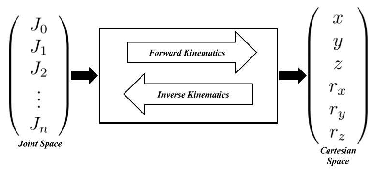
Forward and Inverse Kinematics: Jacobians and Differential Motion

June 20, 2017March 13, 2020Atomoclast 3 Comments

In my last post, we began to scrape the surface in robotic manipulators by discussing joint space, Cartesian space, and their intertwined relationship. The caveat to that analysis was that everything was static. We were solving for end effector position in space or for joint angles given a desired end effector. The issue is, robots have to move with respect to time. Thanks to our good friend Newton, we know as something changes its position with respect to time, we have a velocity.

This robot arm must move in a coordinated fashion to move the gripper into position to catch the object being thrown at it. Source: Swiss Federal Institute of Technology in Lausanne

To make things interesting, sometimes we have constraints on the task at hand that requires to manipulator to move the end effector in a straight line in Cartesian space, think about a task like sliding open a window, or pulling a peg out of a hole like the robot below is about to do. That means just planning joint angles for a starting and ending position isn’t enough, we will need to use coordinated motion between the individual joints to get the resulting end effector to move along a specific path.

This robot will need to use Cartesian control to pull the peg out in the horizontal direction only. Source: MIT CSAIL

Team Jacobian: The Differential Relationship

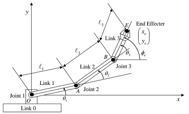
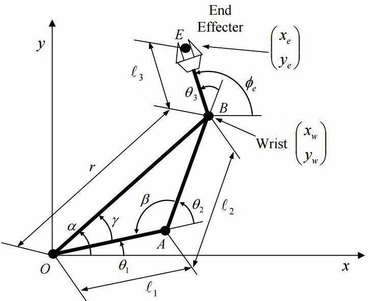
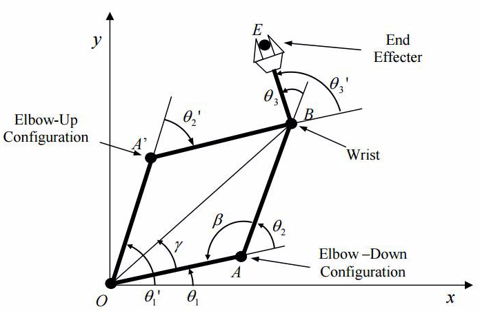
In the last post, we analyzed a planar robot manipulator with three degrees of freedom. To make things a bit simpler on ourselves, we’re going to look at a two degree of freedom manipulator.

Two Degree of Freedom Planar Manipulator, Source: Introduction to Robotics, H. Harry Asada

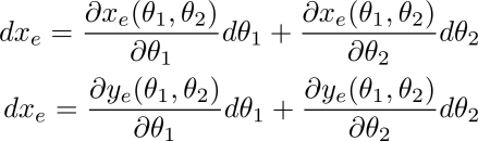
We can then describe the end effector position, xₑ and yₑ, in space in terms of the joint angles θ₁ and θ₂ as follows:

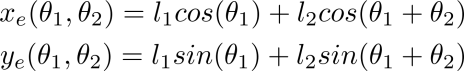
These two linear equations show that any change in either θ₁ or θ₂ will cause a change in xₑ and yₑ. Another way to think of it is that the end effector position is dependent on the variables of the joint angles. Recalling some calculus, we can take the partial derivatives of the above equations and describe the differential relationship between end effector position and joint angle as such:

We can write the above equation in a much more compact format by stating:

Note that:

,

The q vector is known as the system state. The J matrix is referred to as the Jacobian matrix. A Jacobian, mathematically, is just a matrix of partial differential equations. Since we’re engineers and roboticists, we like to make mathematicians angry and refer to the “Jacobian matrix of a manipulator that describes the velocity of the system and how it affects the end effector’s position” as just the “Jacobian”. Small tangent, sure, I’m only bringing it up to make you, the reader, aware that there are other types of Jacobians, anyways, back to the subject at hand. The Jacobian for the system shown above can is:

As I was mentioning above, the Jacobian represents the change of the end effector’s component position with respect to small changes in each joint angle. Now that we have this, we can begin to really apply some interesting control over our arm! Say that we have a robot arm that welds a joint together, and we need to ensure it moves in a particular straight line, with a very specific speed, we can use our new tool, the Jacobian to provide that level of control! Going back to the 2DOF arm shown above, say that we wanted to move the end effector in the x direction at a specific speed, let’s say to weld a straight line, we can formulate the dynamics of the system as follows:

As can be shown here, the Jacobian maps the relationship between joint velocities and end effector velocities.

Inverse Kinematics of Manipulators In Motion

In my last post, we not only discussed forward kinematics, but also inverse kinematics. That analysis was with a static end effector position and orientation in space. In the scenario described above, for the welding robot’s end effector moving in a straight line at the desired velocity, we can do some linear algebra and isolate the joint velocity matrix and obtain:

One very cool thing to note about this solution is that, mathematically, it can only have one solution, as long as the Jacobian is non-singular. In very mathy terms, a Jacobian drops rank and becomes non-invertible. Basically, the math doesn’t work, and the Jacobian doesn’t solve well, and it can cause the controller to tell the manipulator it needs to be at some impossibly high velocity, and the controller will try and follow suit, causing sometimes catastrophic results. It’s reasons like this that massive industrial robots are always behind huge cages and no humans are allowed into the work area.

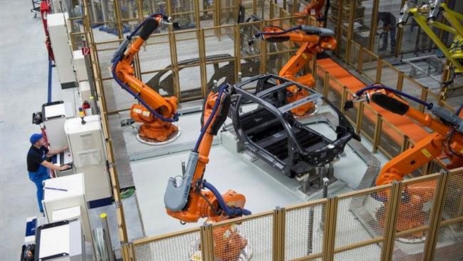
Unfortunately, sometimes industrial robots fail and can cause the loss of human life. This is why collaborative robots (or CoBots) like Universal Robots, have become very popular in recent years. Source: https://www.presstv.com/Detail/2015/07/02/418396/Germany-Baunatal-Volkswagen-Hillwig

If we calculate the inverse Jacobian and multiply that by the decomposed (in terms of component directions) end effector velocity, vₑ, we will have the required individual joint velocities. That means to implement this on a robot, we will command the individual joint controllers to the computed joint velocities, from the above controller. This type of control is called Resolved Motion Rate Control, which can also be shown as:

This is a compact form to implement a resolved motion rate controller given a desired end effector position, and velocity, given feedback on the current position in space. The K term is gain term to help tune the controller.

Since the robot arm’s positions and velocities will change over time, the Jacobian’s computed values will change over time as well, depending on the arm configuration. The take away from this is that some higher level of coordinate will be required to ensure the controller feeds velocities in a smooth and controlled manner.

Let’s look at the above 2DOF arm. We want to move the robot arm from Point A (2, 0) to point B, C, then to finally D (0, 2). Note that each link of the arm below is the same length.

Example 2DOF Arm with desired waypoints for a full trajectory. Notice the curve showing the envelope of maximum reach. Anything along this line would cause a singularity for the arm. Source: Introduction to Robotics, H. Harry Asada

We can now state the joint angles, θ₁, θ₂, as follows:

If we were to graph the joint velocities with respect to time as the arm moved from one point to another, the graph would look as follows:

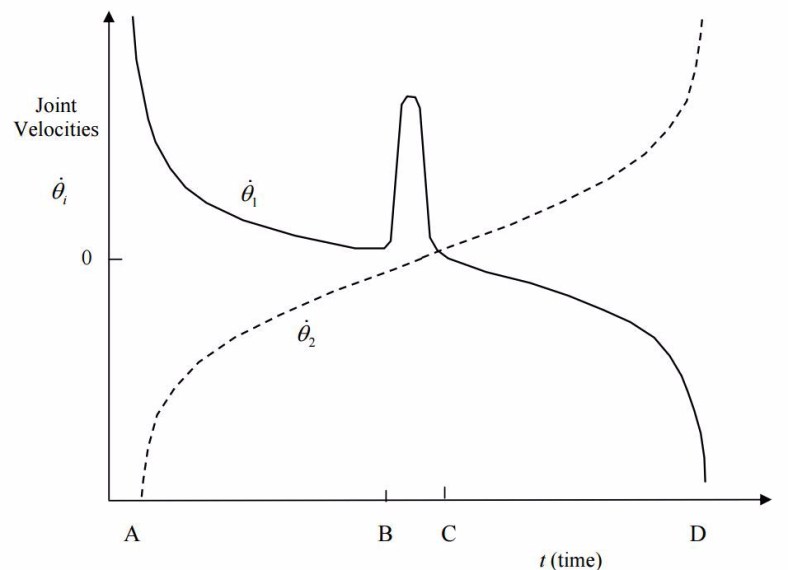
The above graph shows the joint velocities of the arm as it moves through the waypoints with respect to time. Source: Introduction to Robotics, H. Harry Asada

A few things to note in the above graph. First, notice at how large the joint velocities are near the initial and final positions, A and D. This is due to the Jacobian saying that the joint needs to be at a specific position in a short period of time, causing such a high acceleration. In a real system, this could cause a robot to fault due to such high accelerations, another thing that is helping is that at these positions, θ₂ is at or approaching 0. This causes the mathematical issues described above in Jacobian Singularities.

Moving from one extreme to the other, as we approach B, and move to C, we see θ₁ accelerate quickly to allow the end effector to take the shortest path between points B and C. In order to reach this, the joint is almost -180 degrees, which is a singularity for this configuration.

For the interested reader, I highly suggest Stanford’s Intro To Robotics Lectures. The following lecture is about Jacobians in a much finer detail:

Computing Jacobians with ROS

Last week, I showed you how to move a simulation robot from one point in space to another using MoveIt. If you wish to continue with this example, you will need to follow last week’s tutorial and add the proper packages to your catkin workspace.

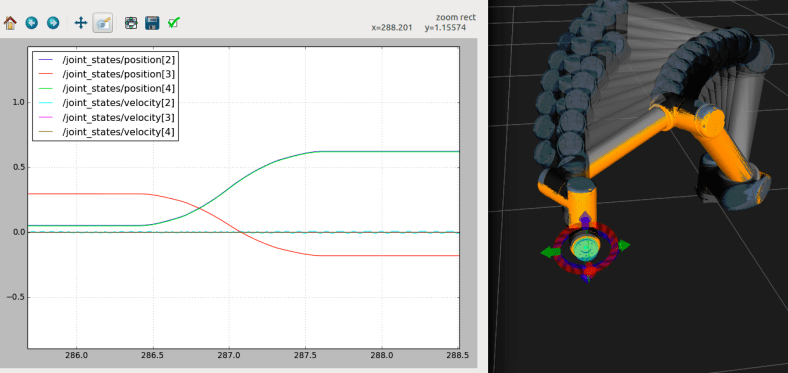
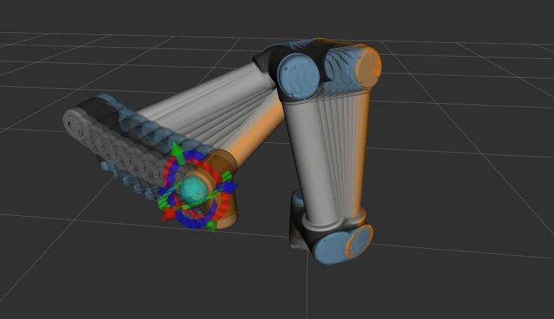
Jacobians are dynamic things. They aren’t easy to visualize like a starting point or an ending point, or even the waypoints in between. They’re intertwined in all of the above, so the only real way to understand them is to experiment with MoveIt and visualize it.

The above image shows a Universal Robot UR10 moving between to waypoints, and a looking at how the velocity profile changes with positions.

To run the above tutorial configuration, you will need to open up four terminals and run:

$ roslaunch ur_gazebo ur10.launch

$ roslaunch ur10_moveit_config ur10_moveit_planning_execution.launch sim:=true

$ roslaunch ur10_moveit_config moveit_rviz.launch config:=true

With that up and running, you should see the same Gazebo Simulation Window as well as Rviz window with the UR being shown and the MoveIt Config window ready for you to plan paths!

In the final terminal you will run:

$ rqt_plot /joint_states/position[2], /joint_states/velocity[2], /joint_states/position[3],/joint_states/velocity[3], /joint_states/position[4], /joint_states/velocity[4]

You can always add or delete which joints you want to track, this is just to get you up and running.

You should then see a window similar to the one in the image above showing the position and velocity of joints as time goes on.

In ROS, most data is exposed as a topic and transferred via messages. We can learn a little more about how ROS encodes these joint state topics by running:

$ rosmsg show JointTrajectory

It should return the structure of a JointTrajectory message:

[trajectory_msgs/JointTrajectory]: std_msgs/Header header uint32 seq time stamp string frame_id string[] joint_names trajectory_msgs/JointTrajectoryPoint[] points float64[] positions float64[] velocities float64[] accelerations float64[] effort duration time_from_start

This is the topic that Rviz/MoveIt and others use to update the virtual robot’s position in space when new information is sent up from a real robot (or our case, a simulation robot, but to our control software, it’s real).

This next section is going to go over the MoveIt API a bit further to get you more into the trenches with the data available with MoveIt. With that API we will be able to print out the UR10’s Joint states, end effector state in Cartesian space, as well as the Jacobian matrix for this robot! To do so, you will need to navigate back to your catkin workspace and clone the following:

If you are on ROS Kinetic:

$ git clone https://github.com/atomoclast/moveit_tutorials.git --branch ur10_kinetic

If you are on ROS Indigo:

$ git clone https://github.com/atomoclast/moveit_tutorials.git --branch ur10_indigo

You should just build the workspace again, then you should be able to run:

If you are on ROS Kinetic:

$ rosrun moveit_tutorials kinematic_model_tutorial

You should then see something similar to my screen:

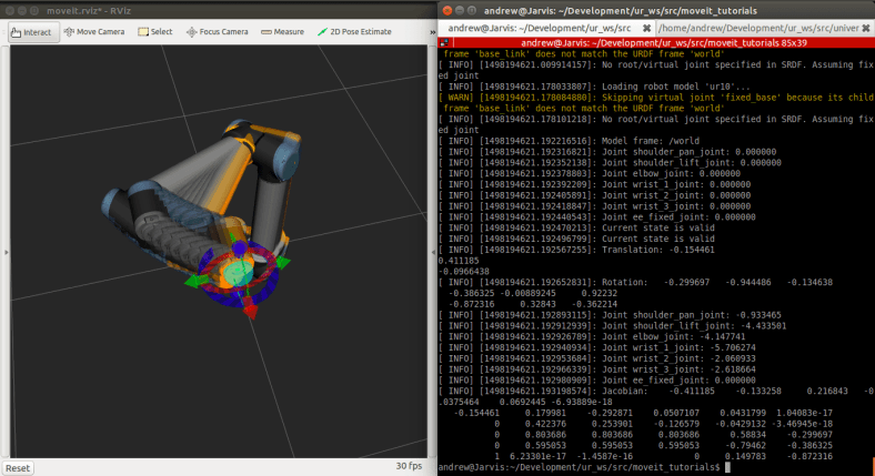
Expected output from the node. Note the Jacobian Matrix on the bottom.

Below is the block of code that is of real interest. It shows how we use the getJacobian() method from the MoveIt API to print the Jacobian.

Eigen::Vector3d reference_point_position(0.0,0.0,0.0); Eigen::MatrixXd jacobian; kinematic_state->getJacobian(joint_model_group, kinematic_state->getLinkModel(joint_model_group->getLinkModelNames().back()), reference_point_position, jacobian); ROS_INFO_STREAM("Jacobian: " << jacobian);

You should try and move the robot in a variety of positions and plans and see how it effects the Jacobian. The matrix is rather large, but as you see, it will be different every time!

Have fun!

For my next post, I’m thinking of some fun computer vision/machine learning projects/tutorials I can post! Stay Tuned!

Liked what you saw? Subscribe for more cool how-tos, side projects, and robot stuff!

Have a comment, issue, or question? Leave a comment or message me on GitHub.

Forward and Inverse Kinematics, an Introduction.

June 16, 2017June 26, 2017Atomoclast 7 Comments

So this will be part one of a multi-portion series of posts. This first post will be very mathematically dense, but if you make it through, it will make the programmatic sections that much more enriched and clear.

While robots come in many different forms from autonomous cars, to drones, and even robots that swim underwater, one thing is for sure, robotic manipulators (arms) are quintessential to the study of any form of robotics. The ability for a robot to convert bytes and electrical signals to effect the world around it is one of the most amazing things about this field. With that in mind, Forward and Inverse Kinematics (FK and IK respectively for the remainder of these posts) are often some of the first things one learns when they start to learn about robotics.

Tesla’s Robotic Charger must use IK to calculate its joint configuration to properly interface with the charging port without crashing.

Before we really sink our teeth into some math, I want to present the concepts of FK and IK conceptually first, because it’s easy to lose sight of what our goals will be when the matrices and notation roll out. I am going to assume that you are reading this on some form of a screen, whether a phone/tablet or a computer monitor. I want to visually look at the top left-hand corner of that screen, and then with your free hand, reach out and touch it with your index finger. While you reach out and touch it, think about how you could have reached it from where you are right now, you probably have enough reach to touch it from the top, or the left side, maybe even perpendicular from the front side of the screen. Thanks to your reach and dexterity, you probably can touch multiple points in the environment around you from a number of ways. A lot of times, robots have the ability to reach several points in space, from multiple angles and joint configurations. This type planning to a particular point in space is what IK is all about.

Source: https://staff.aist.go.jp/eimei.oyama/hpcle.html

Planar Kinematics: Forward Kinematics

Kinematics is the study motion of [rigid] bodies without worry or concern of the forces that caused them or are involved in these motions. We will start off with a really simple example of a planar robotic arm and describe some of the forward kinematics of the arm, which will result in a relationship between a robot’s joints, and where its end effector is in space!

Three Degree of Freedom (DOF) Planar Manipulator with Three Revolute Joints, Source: Introduction to Robotics, H. Harry Asada

The image above shows a serial manipulator, which consists of links of length, that reach from joint axis to joint axis. Each joint has a name of O, A, B, and the end effector (sometimes called tool-tip/frame) is E. With these joints defined, we can now state the length of Link 1 is the distance between joint axis O and A, Link 2 has a length of the distance from A and B, and so on and so forth. If you look at the above image further, you will see that the joints can all rotate around a fixed axis and they will all cause the point, E, to move. We can now state that the position of the end effector in terms of its xₑ and yₑ components. It is also worth stating that this position is with respect to the frame of O. We can then state this relationship between the base frame and end effector frame as such:

We can validate the above equation through derivation and matrix multiplication. If you are new to matrix math and matrix representation of equations, particularly with respect to frame transformations, I highly suggest you check out this chapter from Springer’s Robotics textbook for a detailed description. For a quick recap though, we can state that the rotation, R, around the Z axis as such:

Source: https://commons.wikimedia.org/wiki/FIle:Rotation_about_z-axis.png

We can, therefore, state that rotation in matrix notation as:

Therefore, by example, we can describe the above planar manipulator as a set of matrix transformations for θ₁, θ₂, and, θ₃ as follows:

Initial Rotation around the Z- Axis of Frame O

Pose of the Second Link, With Respect to the First Link, about Frame A, taking into account rotation and translation thanks to l₁.

Pose of the Third Link around Frame B. Note the inclusion of the length of the link, l₂.

Rotation of End Effector Frame E with respect to the third link. Note that since Frame E can never be anything other than inline with frame B, the value for θ will be zero and simplify to above.

We can now state that the transformation from the base frame to the end effector frame is the multiplication of each of the frame transformations between the base frame and end effector frame, that is:

Note: The letters c and s are cos() and sin().

The last step to arrive back at our initial set of equations is to recall that, the position of the end effector has an x and y component, and that our rotations take place in the z component of each frame, therefore we have:

Which gets us back to:

Planar Kinematics: Inverse Kinematics

In the previous section, we studied the relationship between joint angles and an eventual Cartesian position in space, and therefore we can create a new set of definitions and a subsequent relationship in space. We call the configuration of a robot in terms of its joint angles as “Joint Space” and we call the configuration of a robot with its end effector/tool tip in space as it’s “Cartesian Space” configuration. Below is a good graphic that shows this relationship between spaces and FK/IK.

Relationship between Forward Kinematics and Inverse Kinematics

With this relationship established, we can use the concepts and mathematics developed above to figure out the position of the end effector in space, given that we know the joint angles. The real fun begins now. How do we calculate what joint angles will give us a particular point in space if we want to move the robot to do something interesting. Recall the above planar robot, now let’s try and move to a new point in space:

The 3DOF arm is now going to try and reach a new point in space, which will require the calculation of θ₁, θ₂, and, θ₃. This will then lead to us placing the Frame E at xₑ, yₑ, ϕₑ. Source: Introduction to Robotics, H. Harry Asada

Given the above image, and assuming we know what the wrist orientation, ϕₑ, is at, we can simplify the transformation from point E with respect to O as follows. First, let’s recall the earlier results for the transformation from T1 to T4. We can simplify that by dropping off the last length, l₃, since we know what orientation we want the wrist to be in via the variable ϕₑ. We can go back and solve for the last joint angle after we have the other two joint angles. Therefore we can state that:

and state that:

Setting those two together, gives us these equations:

We can square and add the expressions for xₑ, and yₑ and obtain:

We can continue to solve for cos(θ₂) and get:

Note, depending on which sign you decide for the sine function, will give you two different solutions. More on that later.

One down, three to go! We will now solve for θ₁:

It should be noted that if our x and y values are equal to zero, that leads to something called a singularity. The math just doesn’t work out and it doesn’t have a solution.

Now that we have these two angles, we can go back and solve for the last angle!

There it is, that would be a valid solution in joint space to reach the desired position in space. A few things to note though. First off, as we were calculating the second joint angle for Frame A (θ₂), I mentioned that depending on if we picked the positive or negative sign, it will affect the rest of our solutions, the image below shows two valid solutions due to the nature of the math, but with different signs. This type of situation is often addressed by either some level of a cost function, dependent on the initial state of the robot, to either pick the shortest path, OR if an obstacle is in the way, and the system and perceive it, to plan around it/not view it as a valid solution.

Another thing, there was a warning about joint space… if you try and run IK solutions and end up with joints in line with other joints like θ₁ could have been if it were zero, it will result in a mathematically impossible solution. Even if the robot can physically reach it, the numbers don’t play well. Just something to keep in mind.

This figure shows the possibility of multiple solutions. Source: Introduction to Robotics, H. Harry Asada

In closing, this was a very simplified example in reality. Robot arms come in 6 or 7 Degrees of freedom and operate in 3D space, making it very difficult to show without some level of computational assistance and visualization… Let’s go look at something fun!

Computational Inverse Kinematics with ROS

To those who followed this post, this is the benefit of your hard work! The featured image above shows a Universal Robot (UR) planning a trajectory from one point in space to another. I am using a path planning/IK solver called MoveIt! which is a fantastic and flexible open-source package that you can use in the ROS ecosystem to plan complex robot actions. What I will be doing today is showing you how to download the standard UR packages, and use MoveIt alongside a physics simulator named Gazebo to plan some trajectories! Granted what I’m showing you here should be taken with a grain of salt. There is a lot of stuff going on under the hood, but you should at least have a better idea of some of the things that are happening thanks to FK/IK!

I begin by assuming that you will have installed ROS in its entirety as I continue with this tutorial.

First, you’ll need to clone the repo and build the repo into your Catkin Workspace by running:

$ git clone -b YOURDISTRO-devel https://github.com/atomoclast/universal_robot.git

Once that’s done, you will need to then open three terminals and launch the following three commands:

$ roslaunch ur_gazebo ur10.launch

$ roslaunch ur10_moveit_config ur10_moveit_planning_execution.launch sim:=true

$ roslaunch ur10_moveit_config moveit_rviz.launch config:=true

With everything running properly, you should see two screens open as shown in the gif above, one Gazebo simulation window, the other for Rviz. Gazebo, for all intents and purposes, is a real robot to ROS and MoveIt!, which is fantastic, because we will be trying to run it like a real robot. Simulation is an important part in modern robotics because it allows us to abstract, develop, and test higher level control without having to worry about the normal hardware gremlins that always crop up, like having emergency stops needing to be watched, and issues with the lower level controls.

In the RVIZ Window, you will need to select a Planning Library, I suggest RRTConfig, that planner works well with these arms. In future posts, I will get into planning methods and types. It may be worth checking out different planners and trying them out.

Once your planner is picked, select the Planning tab, there you will be able to grab the little orb on the tip of the robot arm, which is called an Interactive Marker. From there, you can grab it and move it freely and see the virtual robot follow, you can grab the arrows and move it in component directions and you can even grab the curved sides and change the orientation of the marker.

When you have the arm in a place you want to try and plan to, you can hit the “Plan” button, see a preview of the trajectory, then hit “Execute” and watch the Gazebo Sim as it moves!

After you’re done with that, you can play around with different configurations between planners as well as starting and ending points for the end effector. The curious reader can even follow some of the MoveIt Tutorials, and learn some more!

In my next post, I will begin to explain Jacobians, and look at MoveIt Python API to allow us to have some real control over our UR Robot! Until then, Happy Tinkering!