
Hey strangers! I know it has been a while since you last heard from me. A lot has been going on the last six months or so…I moved halfway across the country to start a new robotics job and I also got accepted and began an MS program online with Georgia Tech! Needless to say, I’ve been a bit swamped with all of that. I’m back now with an interesting post that started as a school project and has now developed into a side project due to my interest in the subjects related to the Structure from Motion problem.
In several of my previous posts, on path planning and state estimation, I began to mention the SLAM (Simultaneous Localization and Mapping) problem in robotics, which is often considered one of the cornerstones in truly autonomous robotics. SLAM is a very complex problem, and this post is barely going to scrape the surface of it, but I will begin to talk about the mapping portion of SLAM by talking about the Structure from Motion algorithm that has been used in many different applications outside of just robotics, such as GPS applications such as Google Maps, and surveying with drones for visual inspection. Let’s begin!

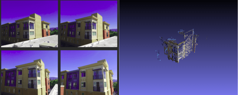
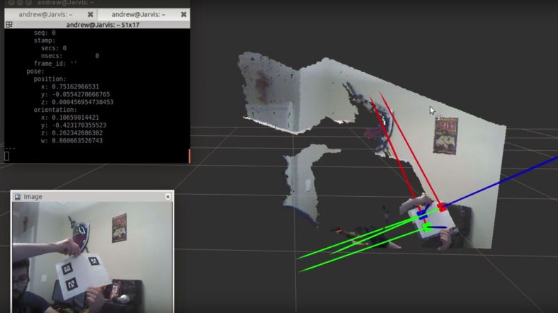
This is an example Pointcloud that was generated using the four images on the right.
Pinhole Camera Model
To begin this discussion, I’m going to quickly go over the pinhole camera model. This is just to explain some important jargon that is required for us to talk about converting things from physical space into images. Camera’s were conceptually conceived via the concept of the camera obscura, which means “dark room” in Latin, really showcases how light from a scene can enter a singular point of entry, the pinhole, and produce a virtual image on the other side of the wall.

An example illustration of a Camera Obscura. Source: https://www.photoion.co.uk/blog/camera-obscura/
I only bring this up, because the modern camera model we use in computer vision is not far from this simple physical phenomena. The image below details the process of how a real point/feature in space get transformed into a pixel in an image:
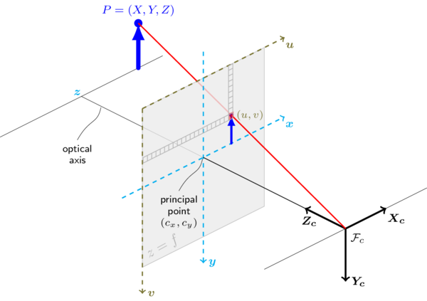
The blue arrow, P, represents some point in Cartesian Space that produces some pixel, (u,v) in our image. This point in real space gets translated into the pixel in our image via the intrinsics of the camera: the focal length of the lens, field of view and the distortion of the physical lense (nothing is ever manufactured perfectly) Source: https://docs.opencv.org/2.4/_images/pinehole_camera_model.png
We can describe this process mathematically as follows:

This equation is the basic format of the pinhole camera model. It relates 3D points to 2D pixel space. Note that R and t are a 3×3 rotation matrix and a 3×1 translation matrix respectively.
The first matrix on the right-hand side of the equation is referred to as the camera’s intrinsic parameter matrix. This has the focal length in vertically and diagonally via the f parameters and the optical center of the image cx and cy. This matrix describes the camera’s physical properties in “pixel” coordinates. The cx and cy values are the pixel values in the image that sit along the optical axis above. More often than not, it is pretty close to half the pixel width and height respectively, but due to manufacturing tolerances, it may not be exactly in the center of the image due to radial distortions as shown below. The focal length expressed in pixels is derived from the field of view and the lens’ physical focal length. One can obtain a camera’s intrinsic calibration matrix using a calibration process with a known checkerboard pattern as detailed in this tutorial.
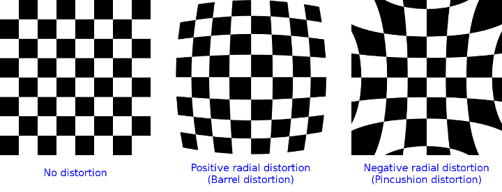
Example of radial distortions from imperfect lenses. Source: https://docs.opencv.org/2.4/_images/distortion_examples.png
The [R|t] portion of the above equation is often called the joint rotation-translation matrix, which is also referred to as the “extrinsic” parameters of the model. We can think of the intrinsic calibration as the “internal parameters” to the camera and the “extrinsic parameters” as the “external” configuration of the camera. So this relates our camera back to a pose in space. You can find more information about rotation matrices and translation matrices in my kinematics tutorial if you want a refresher. Fundamentally, the rotation-translation matrix correlates a point (x, y, z) to a coordinate with respect to the camera. You can find a great write up on the OpenCV website via this link for more information.
Pivoting a bit, we can now talk about how we can build pointclouds with stereo camera rigs from a theoretical sense to help instill a sense of how we can use these physical camera parameters to build 3D clouds. If we had two calibrated cameras that were pointing the same direction, with some distance between the cameras in a purely horizontal sense, we can actually find interesting features in each pair of images and calculate where that point is in space with some simple geometry.

The ZED Stereo Camera is an off the shelf system from StereoLabs. Source: http://www.stereolabs.com
Now if we found an interesting feature in the left image and right image, we can use triangular relationships to find how far that feature is from the camera as shown below. While this is a simplification of the process, it shows how the parallax phenomena helps us calculate differences between the images to build our triangle. Parallax is when you find a feature in two images, but their horizontal locations are different, meaning that they’re along the same vertical line, but not the same horizontal line. You can observe this quickly by holding your hand out in front of your face, and close one eye while leaving the other eye open then swapping. You will see your hand seems to “shift” from the left or right as your switch eyes. For more detail on the mathematics and mechanics of stereo, follow this link.
A simple example of stereo camera triangulation. Source: https://www.cs.auckland.ac.nz/courses/compsci773s1t/lectures/773-GG/topCS773.htm
Recovering Camera Poses
In the above section, we began to detail how a camera’s pose (position and orientation) in space as well as it’s internal parameters produces discrete images for us. We then went over how we can find a point in 3D space with two cameras taking two different images. Structure from Motion operates in the same manner at a high level, but instead of having two images taken at the same time, with some distance between them, we will try and reconstruct these points by finding these matching keypoints between two images that were taken from different positions at different times. We essentially try to build a time-varying stereo camera rig!
So how do we do this? Well, we can do this two ways: by comparing each image with every other image in an image stack, or by using a video stream (think from a small robot or drone) and tracking keypoints as they move between sampled frames using optical flow. For my current example, we used an unsorted approach, where each image was compared against the others, and that’s how I will continue to describe it. I do think that optical flow is how I will probably improve my approach so I can use it with my drone in the future, but I digress.
Comparing each image in an image stack with another is the approach that was originally used in the Photo Tourism research paper published in 2006 that resulted in a software package known as Bundlr. This approach attempts to find matches between images, and then recover a camera’s pose in space by estimating the Essential Matrix via matched features, as shown below. This matrix is a 3×3 matrix that relates the points in the two images and from there, we can calculate the Fundamental matrix, which is what we really care about because it returns to us a rotation matrix, R, and a translation matrix, t.
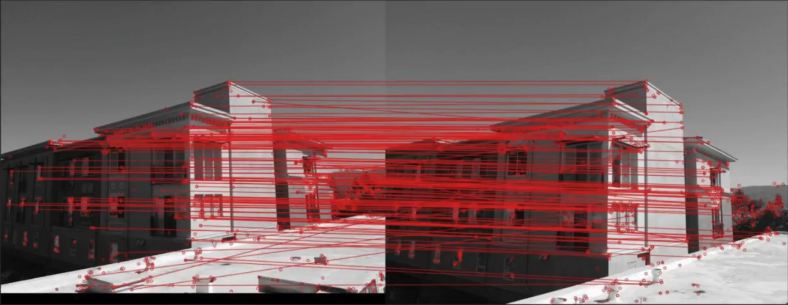
Matches found between two images of the building scene from the example above.
We can recover these points in space because we already know some stuff about the camera: the focal length and the principal point (cx and cy). Since the focal length and optical center of the image are based on real physical measurements, and with the pinhole camera model above, we know how physical points are captured as images, we can do some math to try and solve for what these points are in space.

Where:
- x and x’ is the (u, v) pixel location of the keypoint in the first image and second image respectively.
- K is the calibration matrix consisting of the focal length and principal point coordinates of our camera.
- E is the Essential Matrix
We use a Singular-Value Decomposition (SVD) method to solve the above equation. An interesting note to be made: there are a few methods to calculate the essential matrix, a 5-point method, and an 8-point method that uses 5 and 8 point pairs respectively. Algorithms such as RANSAC (Random Sample Consensus Algorithm) can provide many more pairs and help us have a more robust solution by having more points to triangulate on.
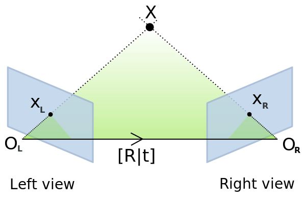
Graphic visualizing the Essential Matrix between two images. Source: imagine.enpc.fr/~moulopn/openMVG/Essential_geometry.png
In the implementation shown in the example above, a 5-point method is utilized to estimate the essential matrix, and that comes with the caveat of ambiguity in the scale of our images. At the end of the day, we won’t know the scale of the differences between images with respect to physical translations so our pose estimate will be relatively correct because or orientations are correct, but we can get around this by making the assumption that the “scale” factor is what is calculated between the first image pair. Note that this is a major drawback to using SfM for map building for motion planning and so on in robotics. There will need to be some external sensor that is utilized for some form of sensor fusion to recover this scale such as an IMU.
Bundle Adjustments and Triangulation
When we used the essential and fundamental matrices to estimate our pose in space, we did it with keypoints, while this is sufficient when we take two images, we haven’t leveraged the constraints that arise when we compare every image with each other and the features that are matched across every image in the image set, for example, the building above has a large overlap in matching keypoints that can improve our statistical confidence in our derived poses in space. This is where the bundle adjustment comes into play! What a bundle adjustment does is treats the entire problem space as a giant nonlinear least-squares problem! Where we try and take the camera poses, the 3D points we can match between the images, and intrinsic matrix, K, and compare them with every other image in the image stack and arrive at one singular solution that is true across all images. Again, to keep this post high level and conversational, I won’t get into the underlying mathematics, but one of the most popular methods is the Levenberg-Marquardt Method. Now thankfully for us, there are a number of libraries that have this implemented for us so this really simplifies the problem for many developers and users like us! Two bundle adjustment library options are SBBA and GTSAM.
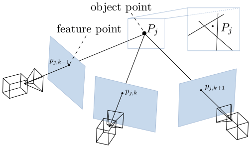
Point Triangulation across multiple images. Once we find our poses in space, optimize our estimates of those poses via a bundle adjustment, we can then triangulate matches in space to build up a high density pointcloud for us to reconstruct a scene from images! Source: imagine.enpc.fr/~moulonp/openMVG/Triangulation_n_geometry.png
Once we’ve optimized our poses in space, we can now triangulate these points in a (hopefully) dense pointcloud artifact! To triangulate these points, we use these known camera poses, our scale factor, and matches to produce our 3D points. A popular way to produce these files is to use a program called PMVS, which is used by Bundlr and several other pointcloud generation pieces of software.
A Structure from Motion Pipeline in C++
As shown above, I have begun to tinker around with a SfM pipeline and have used it on a few image sets with some varying results. You find the source code over on my github.
The software pipeline is as follows:
- Estimate Camera Intrinsics
- An initial camera intrinsic matrix is required as arguments for the main cSfm executable. While one can calibrate a camera or use images from a calibrated camera with known intrinsic, I wanted to keep it flexible enough for any type of images to be passed into the main pipeline of the code. For most of my own images from my own camera, I assumed the center of the image was the width and heights divided by two. I then wrote a simple Python script that takes in the width of the image, the focal length in mm, and the Field Of View to estimate the focal length in pixel space. The code can be found in calculate_focal_length.py
- Find Keypoints in each Image
- From this point on, this is all automatically computed in the compiled C++ executable. Iterate through N images, and find keypoint matches in the rest of the N-1 images. Store these keypoints in a Structure for Motion Object used to ensure that every keypoint that is found is tracked throughout the pipeline of the images. As can be seen, there are a number of good matches, but some false-positives as well.
- Triangulate Points Between Images
- Using OpenCV, we then used these maps of vectors to triangulate the camera poses from matches between images, then we can use those poses to recover structure. Via triangulation. First, we find the Essential Matrix, which helps us calculate the point correspondence between two poses at the same point in space by finding the translation and rotation [R | t] from the second camera with respect to the first. The OpenCV function cv::findEssentialMat is utilized. We then take that matrix to find our poses in space using cv::recoverPose.Since this is a monocular approach, our rotation will be correct, but the scale will probably be off, so we find our scale by calculating vector length between matching keypoints. This is done while we use the cv::triangulatePoints function.
- Bundle Adjustment (BA)
- BA is the parallel process of refining triangulated points in space as well as the camera poses in space. It is a refinement process that helps us make coherent sense of the camera poses in space with some statistical confidence due to the inherent stochastic nature of our sampling. The way we go about this is to use the camera points we triangulated and the poses we recovered. While there are a number of algorithms that can be used, the Levenberg-Marquardt algorithm is one of the most popular, and GTSAM provides a very fantastic implementation of it via: gtsam::LevenbergMarquardtOptimizer
- Prepare Post BA Camera Estimates for PMVS2
- Once the bundle adjustment has been run on all of our triangulated points and poses, we will prepare those estimates in a format for PMVS to use. This requires several system calls to produce directories and populate them with images in the format that PMVS expects, and the corresponding Projection Matrix. This P matrix is what relates the camera with respect to an origin coordinate in space.
- Utilize PMVS to create the Pointcloud
- Patch-Based Multi-View Stereo is its own compiled piece of software, but it is automatically called via system calls in the cSfM executable. It looks in the local directory for the output/ directory that was generated in the last step, and takes those Projection matrices and the corresponding images, and stitches them together into the final pointcloud .ply file.
Building the Software
To build it, you will need to have GTSAM setup on your local machine. I used version 4.0.0-alpha2.
To clone it locally on a Linux machine by running,
git clone https://github.com/atomoclast/cSfM.git
From there navigate to the root of the directory:
cd path/to/cSfM
and build the executable by running:
mkdir build

cd build

cmake ..

make
You should then see a cSfm executable now in the build directory.
Usage
To use cSfM, you will need to have a directory containing several images of your item of interest. You will also need to pass in the FULL path to a text file that contains the name of the images in the same folder you wish to build the pointcloud of, the focal length of your image (in pixels), the center of your image in x and y.
If you are using a calibrated camera, this should be easy to find as elements in the resultant distortion matrix.
However, if you are using images from a smart phone/uncalibrated camera, you can estimate these parameters.
To calculate the focal length of your image, I have written a simple helper Python script. The way you use that is as follows:
python calculate_focal_length.py [pxW] [f_mm] [fov]
where:
pxWis the width of the images in pixels.f_mmis the focal length of the camera that was used to capture the image in [mm].fovis the camera’s Field of View in degrees.
To get this information, one can look at the EXIF metadata that their images should have.
This should print out a relatively accurate estimate of the focal length of your images in pixel space.
For a rough estimate of the center of the image in x and y, you can use this rough estimate:
- cx = PixelWidth/2
- cy = PixelHeight/2
This should be accurate enough, as the algorithm will attempt to calculate a more accurate camera matrix as it triangulates points in space via the bundle adjustment.
Assumptions and Caveats
This is still a first attempt at SfM. SfM is a very complex problem that still has a lot of research conducted on how to use different cameras and different improve results. That being said, here are some thoughts and tips to get good results:
- Scale down your images. This pipeline does not use a GPU based method to calculate poses in space via triangulation, so it may take a long time.
- Try and use images that have large overlaps in them. Right now the pipeline matches keypoints across all the images, so if there is not enough overlap, it will struggle to recover camera poses.
- Use a few images at first to test things out. Do not overestimate how computationally expensive it becomes as the size of images and volume of the image stack increases.
Examples and Results

This was one of the first simple image sets I used to test and debug my code. It is a corner of my desk at work. I figured the contrasts in colors helped with debugging false positives for
Link to video with rotating pointcloud.

This was an small group of photos taken of our Harry Potter Book Collection with some Harry Potter Bookends.
Link to video with rotating pointcloud.
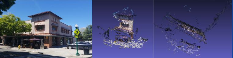
A series of pictures were taken by a local pizzeria. I ran the program with the full image set, and then with only 3 images out of curiosity. The full image set created a much fuller “face” of the building in the left point cloud.. Using 3 images highlighted the right angle of the building as shown in the image on the right. The perspective was taking from the top to show the joining of the front face and the right facade. It would be interesting to see how one can merge Pointclouds in the future.
References
- http://www.cse.psu.edu/~rtc12/CSE486/lecture19.pdf
- https://docs.opencv.org/3.0-beta/modules/calib3d/doc/camera_calibration_and_3d_reconstruction.html
- https://docs.opencv.org/3.1.0/da/de9/tutorial_py_epipolar_geometry.html
- http://nghiaho.com/?p=2379
- https://www.di.ens.fr/pmvs/pmvs-1/index.html
- http://www.cs.cornell.edu/~snavely/bundler/
- https://robotics.stackexchange.com/questions/14456/determine-the-relative-camera-pose-given-two-rgb-camera-frames-in-opencv-python
- https://www.cc.gatech.edu/grads/j/jdong37/files/gtsam-tutorial.pdf
